The KEY Institute for Brain-Mind Research, University Hospital of Psychiatry, Zurich, Switzerland

1. Localization properties of instantaneous, 3D, discrete, linear solutions for the EEG inverse problem
One of the primary concerns in electrophysiology is the non-invasive localization of the neuronal generators
responsible for measured EEG phenomena. Methods for localization are termed inverse solutions. This review is limited
to the class of instantaneous, 3D, discrete, linear solutions for the EEG inverse problem. In order for an inverse
solution of this class to qualify as a true functional "tomography", it must at least be capable of localizing
sources with a minimum of localization error. If an inverse solution of this class is incapable of correct localization,
then it has no worth as a tomography. Harsh as this criterion may seem, it is fair and objective, but most important
of all, it is applicable to any proposed method.
The main difficulty impeding the development of a "good" tomography for the generators of the EEG
is determined by the physics nature of the problem: the measurements do not contain enough information about the
generators. This gives rise to what is known as the non-uniqueness of the inverse solution. Therefore, from the
outset, it can be stated that a perfect tomography can not exist. Despite this obstacle, the search for better
tomographies goes on, as witnessed by the number of papers being published in this field (see, e.g., [8] for a
recent review).
From a more optimistic point of view, one might expect that whatever little information is contained in EEG
measurements, it should suffice to allow for the existence of at least an "approximate" tomography. Such
a tomography should be capable of recovering the "true" generators with an acceptable low level of distortion
(i.e., of error).
Historically, the first tomography published in this field was the minimum norm inverse solution of Hämäläinen
and Ilmoniemi [6]. The properties of this method for 2D solution spaces (i.e., sources restricted to a plane or
to a spherical surface running parallel to the measurement surface) were promising. Two-dimensional images of estimated
current density corresponding to ideal point sources were recovered with blurring, but with correct localization
of activity maxima. However, this method is incapable of correct localization in 3D solution spaces, as was shown
in Pascual-Marqui [10].
The greatest challenge in the development of EEG source localization tomographies is to extend the good localization
properties of the 2D minimum norm solution to 3D solution spaces. This was achieved with LORETA (low resolution
brain electromagnetic tomography)[10,11].
All the properties of a tomography, including its quality in terms of localization capability, can be completely
characterized by means of the model resolution matrix [9,3]. This
approach was used by Pascual-Marqui [10] to compare three tomographies (inverse
solutions) in terms of their localization errors.
The first part of this paper contains a brief review of the theory of instantaneous, 3D, discrete, linear solutions
for the EEG inverse problem. A methodology is presented for the fair, objective, and rigorous comparison of EEG-based
tomographies. The main results presented here correspond to a comparison of five different tomographies taken from
the published literature.
Some important aspects of inverse solutions not included in this study, such as the effect of noisy measurements
and the effect of the reference electrode for EEG measurements, were considered in detail elsewhere
[10]. Other methods of source localization, such as single or multiple dipole fitting are not the object of
this review.
1.1 Material and methods
The forward problem
The "forward" equation, which gives scalp electric potential differences as a function of the current
density (produced by neuronal generators), is:
| |
 |
(1) |
In Eq. (1), Φ is an N1-matrix comprised of measurements of scalp electric
potential differences. The coordinates of the measurement points are given by the Cartesian position vectors  . The (3M)1-matrix
  is comprised of the current densities
  at M points within the brain volume,
with β = 1...M. The super-script "T" denotes transpose. The coordinates of the source points within
the brain volume are given by the Cartesian position vectors
at M points within the brain volume,
with β = 1...M. The super-script "T" denotes transpose. The coordinates of the source points within
the brain volume are given by the Cartesian position vectors  . The N(3M)-matrix K is a transfer matrix. The α th
row of the matrix K, with α =1... N, is
. The N(3M)-matrix K is a transfer matrix. The α th
row of the matrix K, with α =1... N, is  , where
  is the lead
field. For instance, the electric lead field in an infinite homogeneous conducting medium is:
is the lead
field. For instance, the electric lead field in an infinite homogeneous conducting medium is:
| |
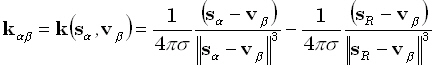 |
(2) |
where σ is the conductivity, and sR
is the position vector to the reference electrode. In the simulation studies for the
EEG case, the average reference lead field equations corresponding to a three-concentric spheres head model will
be used [1] instead of Eq. (2).
The problem of interest here is the case when the M points (voxels) within the brain volume span a true
3D volume. This collection of M points is termed the solution space. It must not be limited to, e.g., points
lying on a spherical surface. Furthermore, the points will be assumed to form part of regular cubic grid. In the
forward problem, Φ is unknown; whereas  ,
,  , K, and J are known. In the inverse problem, only J is unknown, and there are
many more unknowns than equations, i.e., M>N.
, K, and J are known. In the inverse problem, only J is unknown, and there are
many more unknowns than equations, i.e., M>N.
It is not the aim of this review to discuss other forms of the forward equation corresponding to more "realistic"
head models, which take into account, e.g., head shape, anisotropic conductivities, etc. In any case, only the
matrix K above changes, and this has no consequence on the methodological aspects presented in this paper.
Inverse solutions in general
For exact noise-free measurements, any instantaneous, 3D, discrete, linear solution for the EEG inverse problem
can be written as:
| |
 |
(3) |
where the (3M)N-matrix T is some generalized inverse of the transfer matrix K,
which must satisfy:
| |
 |
(4) |
where  denotes the NN
average reference operator, defined as:
denotes the NN
average reference operator, defined as:
| |
 |
(5) |
where  denotes the NN
identity matrix, and
denotes the NN
identity matrix, and  is an N1
matrix comprised of ones.
is an N1
matrix comprised of ones.
Eq. (4) expresses the fact that the estimated current density (i.e., the inverse solution) given by Eq. (3)
must satisfy the measurements in forward Eq. (1).
The EEG inverse problem is known to have infinite solutions. This means that there exist an infinite number
of different generalized inverse matrices T, all producing current densities  (Eq. (3)) that satisfy the original measurements Φ (Eq. (1)).
The resolution matrix
The main question now is: what criteria should be used for selecting a particular inverse solution?, or for
preferring one particular inverse solution to all others? The quality of any given instantaneous, 3D, discrete,
linear inverse solution for EEG can be analyzed in terms of the resolution matrix of Backus and Gilbert
[3] (see also [9]). Substituting Eq. (1) in (3) gives the following relation between
"true (J)" and "estimated ( )" current densities:
| |
 |
(6) |
where:
| |
 |
(7) |
In Eqs. (6) and (7), R is the resolution matrix. In an ideal situation, R is the identity matrix,
and the current density can be estimated exactly. However, for the EEG inverse problem studied here, the resolution
matrices are quite far from being ideal.
There are at least two ways to fully characterize the properties of a given inverse solution, based on its resolution
matrix: by means of the collection of all columns, or of all rows. By definition, both approaches contain the same
amount of information about the inverse solution being studied. In a first approach, the collection of all columns
will be considered. A column of the resolution matrix corresponds to the "estimated" current density
for a "true" point source. This can be seen directly from Eqs. (6) and (7), when the true current density
contains zeros everywhere, except for unity at some given element. The estimated current density in this case is
known as the "point spread function." An exhaustive study of all possible point spread functions constitutes
a complete characterization of an inverse solution, since trivially, the set of all columns of a matrix defines
uniquely the matrix.
The essence of any tomography (i.e., of an instantaneous, 3D, discrete, linear inverse solution for EEG), is
the property of correct localization. Therefore, the only relevant way of testing a linear tomography is to analyze
the estimated images produced by ideal point sources. Such tomographic images are precisely the point spread functions.
If these images have incorrectly located peaks, then the method does not deserve the name of "tomography",
due to the lack of any localization capability.
The second approach that characterizes an inverse solution consists of studying the rows of the resolution matrix,
which correspond to the averaging kernels of Backus and Gilbert [3]. An averaging kernel
contains information about how the current density estimator at some given point is influenced by all possible
sources. Ideally, an averaging kernel should indicate high influence of the source at the point of interest, and
should indicate low influence of all other possible sources. It can be rigorously shown, at least for the EEG problem
in a piece-wise homogeneous medium, that the averaging kernels always attain their extreme values on the borders
of the solution space. The proof of this property is based on the following facts:
1. An averaging kernel is a linear combination of lead field functions.
2. At least in the case of the piece-wise homogeneous head model for EEG, the lead fields are harmonic functions,
i.e.,  .
.
3. A linear combination of harmonic functions is harmonic.
4. Harmonic functions attain their extreme values on the boundaries of their domain of definition
[2].
This property means that, for a discrete 3D solution space for the EEG inverse problem, it is not possible to
even obtain near-ideal averaging kernels at any non-boundary point of interest. In addition, this property demonstrates
the futility of trying to design near-ideal averaging kernels, since it is physically and mathematically impossible
in a 3D solution space.
The non-existence of ideal averaging kernels for non-boundary points gives rise to the fundamental question:
are linear inverse solutions doomed to incorrectly localizing deep non-boundary sources? The results presented
below answer this question, showing that only the LORETA method is capable of localizing these sources, albeit
with a certain degree of under-estimation.
Particular inverse solutions: minimum norm (MN), weighted minimum norm (WMN), and low resolution brain electromagnetic
tomography (LORETA)
There exist at least two possible formulations for deriving some of the linear solutions found in the literature.
Only the average reference EEG problem will be considered here (details for the MEG inverse problem can be found
in Pascual-Marqui, 1995). In one approach, the inverse solution corresponds to a constrained solution of the forward
equation. In this case, the following problem must be solved:
| |
 |
(8) |
for any given positive definite matrix W of dimension (3M)•(3M). The solution is:
| |
 |
(9) |
where  denotes the Moore-Penrose
pseudoinverse of
denotes the Moore-Penrose
pseudoinverse of  .
.
In another approach, the inverse solution corresponds to the generalized inverse matrix T that optimizes, in
a weighted sense, the resolution matrix. The problem statement here is to solve:
| |
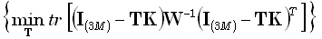 |
(10) |
where  is the (3M)•(3M) identity matrix, and "tr" denotes the trace of a matrix.
Note that the problem in Eq. (10) expresses the minimization of deviation of the resolution matrix from ideal behavior.
The solution to (10) is identically Eq. (9) again.
is the (3M)•(3M) identity matrix, and "tr" denotes the trace of a matrix.
Note that the problem in Eq. (10) expresses the minimization of deviation of the resolution matrix from ideal behavior.
The solution to (10) is identically Eq. (9) again.
The minimum norm solution of Hämäläinen and Ilmoniemi [6] corresponds
to Eq. (9) with  . The weighted
minimum norm solution corresponds to
. The weighted
minimum norm solution corresponds to 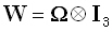 ,
where ⊗ denotes the Kronecker product,
,
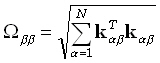
where ⊗ denotes the Kronecker product,  is the identity 33-matrix, and Ω is a diagonal
MM-matrix with
is the identity 33-matrix, and Ω is a diagonal
MM-matrix with
| |
 |
, for β = 1...M. |
The low resolution brain electromagnetic tomography (LORETA) method [10] corresponds to:
| |
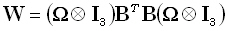 |
(11) |
where the matrix B implements a discrete spatial Laplacian operator. It should be emphasized that such
a choice for B produces the smoothest possible inverse solution. This is because the inverse matrix, i.e.
 , implements a discrete spatial
smoothing operator. For a solution space given by a regular cubic 3D grid, with minimum inter-grid-point distance
"d", the Laplacian operator used in practice is defined as:
, implements a discrete spatial
smoothing operator. For a solution space given by a regular cubic 3D grid, with minimum inter-grid-point distance
"d", the Laplacian operator used in practice is defined as:
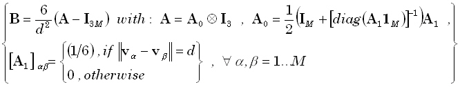
(12)
where 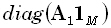 denotes a diagonal
matrix with diagonal elements defined by the elements of the M•1 matrix
denotes a diagonal
matrix with diagonal elements defined by the elements of the M•1 matrix  . Eq. (12) corresponds
exactly to the Laplacian operator implicitly defined and used in Pascual-Marqui [10]
(see Eq. (2'') therein). The explicit definition of the Laplacian is included here (Eq. (12)) for the benefit of
readers that may be interested in implementing LORETA correctly.
. Eq. (12) corresponds
exactly to the Laplacian operator implicitly defined and used in Pascual-Marqui [10]
(see Eq. (2'') therein). The explicit definition of the Laplacian is included here (Eq. (12)) for the benefit of
readers that may be interested in implementing LORETA correctly.
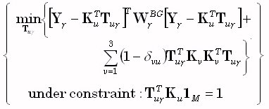
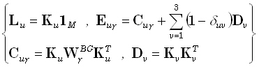
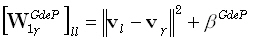
Particular inverse solutions: Backus and Gilbert, and weighted resolution optimization (WROP)
In order to derive these inverse solutions, the forward problem will be rewritten as:
| |
 |
(13) |
In Eq. (13) and in what follows, the subscripts u and v will take integer values (1,2,3) corresponding
to the Cartesian vector field components (x,y,z), respectively. The M•1 matrix
 is now defined
as
is now defined
as  , with similar definitions
for
, with similar definitions
for  and
and  . The transfer matrix
  is now an N•M matrix, with its α th
row (for α = 1...N) defined as
is now an N•M matrix, with its α th
row (for α = 1...N) defined as  . The matrices
  and
and  are defined
similarly. It should be noted that Eqs. (1) and (13) are identical.
are defined
similarly. It should be noted that Eqs. (1) and (13) are identical.
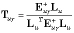
Any linear inverse solution for a field component is of the form:
| |
 |
(14) |
where the generalized inverse  is an M•N matrix. The linear inverse solution at the γ th grid point (γ = 1...M),
for the u th field component, is:
is an M•N matrix. The linear inverse solution at the γ th grid point (γ = 1...M),
for the u th field component, is:
| |
 |
(15) |
where  denotes the γ th
row of
denotes the γ th
row of  .
.
Substituting (13) in (15) gives:
| |
 |
(16) |
| |
 |
(17) |
is the averaging kernel. According to Backus and Gilbert [3], the "best"
inverse solution must make the 1•M vector  be as similar as possible to
  , where δ is the Kronecker delta, and
 denotes the γ th
column of the M•M identity matrix. Note that
denotes the γ th
column of the M•M identity matrix. Note that  corresponds to the discrete representation of the Dirac delta. The Backus and Gilbert problem
[3] was stated as:
corresponds to the discrete representation of the Dirac delta. The Backus and Gilbert problem
[3] was stated as:
| |
 |
(18) |
The constraint in (18) is termed the unimodularity constraint. One choice for the M•M diagonal matrix  is:
is:
| |
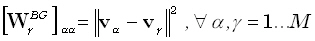 |
(19) |
The solution to (18) is:
| |
 |
(20) |
| |
 |
(21) |
Note that Eq. (20) must be calculated for all vector field components (u=1,2,3), and for all grid points
of the solution space γ = 1...M).
It is important to emphasize that the Backus and Gilbert inverse solution based on Eq. (20) does not satisfy,
in general, the measurements in the forward equation.
The weighted resolution optimization (WROP) method of Grave de Peralta Menendez et al. [5]
corresponds to the solution of the following problem:
| |
 |
(22) |
where  and
and  are diagonal M•M matrices defined as:
| |
 |
(23) |
| |
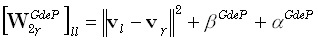 |
(24) |
where  is a scalar, and in
the particular case considered here,
is a scalar, and in
the particular case considered here,  is also a scalar.
The solution to (22) is:
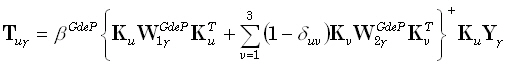 |
(25) |
Several comments on the WROP solution are in order:
1. The article by Grave de Peralta Menendez et al. [5] omitted an explicit equation of
the inverse solution for the case of an unknown vector field. The explicit Eq. (25) is included here for the benefit
of readers that may be interested in implementing and testing the WROP method.
2. The WROP inverse solution does not satisfy, in general, the measurements in the forward equation.
3. Eq. (25) for the WROP method is incorrect for the MEG inverse problem in a spherically symmetric head model.
A correct equation must take into account that the estimated current density is exactly a tangential vector field.
4. In the paper by Grave de Peralta Menendez et al. [5] there is no indication about how
to determine or select the WROP parameters. In view of this situation, values of 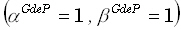 are used in the simulation studies performed in this paper.
A comparison of tomographies: to localize or not to localize
The aim of a tomography is localization. For this reason, as a first comparative test of tomographic methods
for EEG, the main (and only) property of interest is the localization error. As explained previously, all the information
on localization error of a tomography is given by the set of all columns (all point spread functions) of the resolution
matrix (Eq. (7)).
Referring to Eq. (6), consider an ideal "true" point source defined as  , where
  is the α th
column of the (3M)•(3M) identity matrix. The location in 3D space
for the α th
voxel is
is the α th
column of the (3M)•(3M) identity matrix. The location in 3D space
for the α th
voxel is  , where "c"
(taking values in the range 1...M) is given by:
, where "c"
(taking values in the range 1...M) is given by:
| |
 |
(26) |
where "int[r]" denotes the "integer part of r". From Eqs. (6) and (7), the corresponding
3D tomographic image is given by:
| |
 |
(27) |
which is the α th
column of the resolution matrix (or point spread function). The least of all properties that a tomography must
possess is that images of point spread functions have their maxima located as correctly as possible. This property
is a necessary (although not sufficient) condition for correct localization in general. The location of the point
spread function maximum is  ,
where:
,
where:
| |
 |
(28) |
and:
| |
 |
(29) |
In Eq. (29) the set  consists
of all elements of the (3M)•1 matrix given by Eq. (27).
consists
of all elements of the (3M)•1 matrix given by Eq. (27).
The localization errors for testing a tomography are defined as the set of values:
| |
 |
(30) |
for all point spread functions. This test was fully explained and used in a fair and objective comparative study
of several inverse solutions [10].
The head model
Simulation studies in this paper will be based on implementing the five inverse solutions previously described
(MN, WMN, LORETA, Backus and Gilbert [3], and WROP), for average reference EEG measurements
corresponding to a three-shell spherical head model [1] of unit radius sphere. The measurement
space consists of 148 electrodes lying on the scalp surface. The locations used here were adapted from coordinates
provided by Lütkenhöner and Mosher (private communication), and are illustrated in Fig. 1. The solution
space consists of 818 grid points (voxels) corresponding to a 3D regular cubic grid with minimum inter-point distance
d=0.133, confined to a maximum radius of 0.8, with vertical coordinate values z3-0.4. Fig. 2 illustrates the solution space by means of a collection of horizontal slices through the brain.
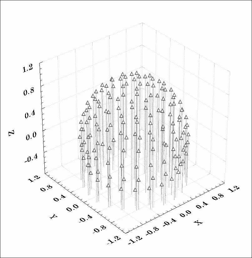
Figure 1. 3D representation of the measurement space defined by 148 scalp EEG
electrodes. A unit radius, three-concentric spheres model is used for the head.
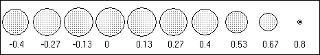
Figure 2. Solution space consisting of 818 voxels (shown as dots) corresponding to a
3D regular cubic grid with minimum inter-voxel distance d=0.133, confined to a maximum radius of 0.8, with vertical
coordinate values z3 -0.4. Numbers below each horizontal "brain"
slice indicate the Cartesian "z" coordinate. Coordinate origin is at sphere center.
1.2. Results and discussion
Fig. 3 shows localization errors as defined by Eq. (30). In each row, the set of horizontal tomographic slices
through the brain corresponds to a different inverse method. Localization errors are gray-color coded in the slices,
with white indicating zero localization error, and black indicating 7 or more grid units of localization error.
A localization error of 1 grid unit means that the point spread function had its maximum only 1 voxel away from
the correct position. This result shows that only LORETA has an acceptable low localization error of 1 grid unit
in the average. All other methods (Backus and Gilbert [3], MN, WMN, and WROP ) are incapable of localizing non-boundary sources. In this respect,
they are similar to x-rays, and can not be qualified as tomographies, since they offer no depth information at
all.
) are incapable of localizing non-boundary sources. In this respect,
they are similar to x-rays, and can not be qualified as tomographies, since they offer no depth information at
all.
Furthermore, a detailed quantitative analysis of LORETA localization errors for boundary sources (i.e., sources
on the border of the solution space) showed that out of 819 cases, a correctly implemented LORETA method localizes
383 cases with zero localization error (47%). Another 356 border points (44%) are localized with 1 grid unit of
localization error.
Fig. 4 illustrates the performance of two tomographies, LORETA and WROP, when confronted
with the task of localizing two simultaneous point sources, one of which is very deep. The tomographic slices in
Fig. 4 do not show localization errors, as was the case in Fig. 3.
The tomographic slices in Figs. 4B and 4C show, in a gray-color coded scale, the estimated current density, with
white indicating zero, and black indicating maximum current density. The locations, orientations ("mom"),
and strengths of two simultaneous test sources are shown in Fig. 4A. The LORETA slices in Fig. 4B show the estimated
current density for each field component ([X-comp], [Y-comp], [Z-comp]) and for field strength ([Strength]). In
contrast to LORETA which can localize both sources correctly (albeit in a blurred fashion), the WROP method in
Fig. 4C is incapable of correct localization. The incapability of correct localization of the WROP method, as shown
in Fig. 4, is shared identically by the minimum norm, the weighted minimum norm, and the Backus and Gilbert methods.
The capability of correct localization of the LORETA method, as shown in Fig. 4, was confirmed for many test sources
(single and double), with locations randomly generated.
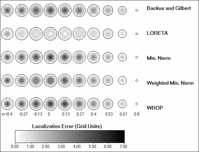
Figure 3. Localization errors for all tomographies. Horizontal slices in each
row correspond to different inverse methods. Localization errors are gray-color coded (white= zero localization
error; black= 7 grid units of localization error). A localization error of 1 grid unit means that the point spread
function had its maximum only 1 voxel away from the correct position. The WROP method implemented here had parameter
values of  .
.

Figure 4. Estimated current density for the LORETA and the WROP methods. (Note
that these slices display current density and not localization error, as was the case in Fig. 3.) The task in this
case was to localize two simultaneous point sources, one being very deep. The locations, orientations ("mom"),
and strengths of the two simultaneous tests sources are shown in (A). Estimated current density is gray-color coded
[white= zero; black= maximum]. The LORETA slices in (B), and the WROP slices in (C), show the estimated current
density for each field component ([X-comp], [Y-comp], [Z-comp]) and for field strength ([Strength]).
The higher strength value assigned to the deep test source in Fig. 4A was chosen to approximately achieve equal
powers of the scalp EEG measurements of both sources. LORETA fails to detect the deep source as a distinct estimated
current density maximum, if it is assigned unit strength. The reason is that the deeper the actual source, the
more blurred is the estimated current density with LORETA. In other words, deep sources are, in the worst of cases,
under-estimated with LORETA. In contrast, all other methods (MN, WMN, WROP, and Backus and Gilbert) produce meaningless
and unacceptable estimators for deep sources, even if they are infinitely strong.
The results and tests presented here demonstrate that LORETA in 3D space has good localization properties, similar
to the minimum norm solution applied to a 2D solution space. However, it is obvious that localization capability
must deteriorate when extending the solution space from 2D to 3D, while utilizing the same amount of information
(EEG measurements). It must be admitted that the test for evaluating localization errors does not prove that LORETA
will localize any arbitrary source distribution. However, low localization error, in the sense defined here, constitutes
a minimum necessary condition to be satisfied by any tomography. In other words: an inverse solution is worthless
as a tomography if it does not comply with this minimum necessary condition.
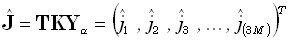
2. LORETA in the human Talairach brain: EEG meets MRI
In this implementation, LORETA made use of the three-shell spherical head model registered to the Talairach
human brain atlas [13], available as a digitized MRI from the Brain Imaging Centre,
Montreal Neurologic Institute. Registration between spherical and realistic head geometry used EEG electrode coordinates
reported by Towle et al. [14]. The solution space was restricted to cortical gray matter
and hippocampus, as determined by the corresponding digitized Probability Atlas also available from the Brain Imaging
Centre, Montreal Neurologic Institute. A voxel was labeled as gray matter if it met the following three conditions:
its probablity of being gray matter was higher than that of being white matter, its probablity of being gray matter
was higher than that of being cerebrospinal fluid, and its probability of being gray matter was higher than 33%.
Only gray matter voxels that belonged to cortical and hippocampal regions were used for the analysis. A total of
2394 voxels at 7mm spatial resolution were produced under these neuroanatomical constraints. A software package
(executables and data) implementing LORETA in Talairach space is available upon request from the author.
Figure 5 illustrates LORETA images of neuronal electric activity in Talairach space.
The recording, corresponding to a visual event related potential during word stimulation (data included in the
software package), was kindly provided by Koenig and Lehmann [7]. LORETA was computed at
the P100 peak. 21 electrodes (10/20 system) were used.
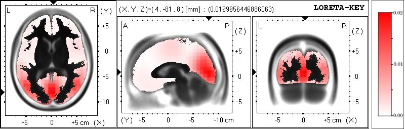
Figure 5. images of neuronal electric activity computed with LORETA.
The images display the neuronal generators of the P100 visual evoked potential peak during word stimulation. Activity
is gray-scale coded (right side inset), with white for zero and black for maximum. Three orthogonal brain views
in Talairach space are shown, sliced through the region of the maximum activity. Structural anatomy is shown in
black outline. Left slice: axial, seen from above, nose up; center slice: saggital, seen from the left; right slice:
coronal, seen from the rear. Talairach coordinates: X from left (L) to right (R); Y from posterior (P) to anterior
(A); Z from inferior to superior. The location of maximum activity is given as (X,Y,Z) coordinates in Talairach
space, and is graphically indicated by black triangles on the coordinate axes. The most active neuronal generators
are distributed in Brodmann areas 17 and 18 (cuneus). Slightly weaker secondary sources are located with bilateral
symmetry at 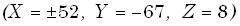 , in associative
cortices, Brodmann areas 37 and 39 (middle temporal and middle occipital gyri). Original images are in color.
, in associative
cortices, Brodmann areas 37 and 39 (middle temporal and middle occipital gyri). Original images are in color.
Ideally, LORETA computations should use the exact head model determined from each individual subject's MRI.
The final step in any analysis procedure would be to cross-register the individual's anatomical and functional
image to the standard Talairach atlas. The main flaw of the procedure presented in this paper is the use of an
approximate head model. However, it has been shown [4] that with as little as 16 electrodes,
and using the approximate three-shell head model, human in vivo localization accuracy of EEG is 10 mm at
worst. Consequently, it can be safely assumed that, given the 7 mm resolution of the current implementation of
LORETA-TALAIRACH, localization accuracy is at worst in the order of 14 mm.
An example demonstrating the statistical analysis of LORETA-TALAIRACH images for the comparison of the activity
patterns between schizophrenic and control subjects can be found in Pascual-Marqui et al [10].
References

 Home
Current Issue
Table of Contents
Home
Current Issue
Table of Contents
