|
Comparison of Algorithms for the
Localization of Focal Sources: Evaluation with Simulated Data and
Analysis of Experimental Data
Rolando Grave de Peralta
Menendez and Sara Gonzalez Andino
Functional Brain Mapping Lab.,
Department of Neurology, Geneva University Hospital,
Geneva, Switzerland.
Abstract. This paper presents a
comparative study of the capabilities of five distributed linear
solutions to accurately determine the position of single sources. Two
recently developed inverse solutions, LAURA and EPIFOCUS are compared to
the Minimum Norm, the column Weighted Minimum Norm and the Minimum
Laplacian. The comparison is based on three figures of merit: 1) the
number of sources with zero localization error, 2) the maximum
localization error, and 3) the average localization error as a function
of the source eccentricity. The best results in terms of the three
figures of merit are obtained for EPIFOCUS and LAURA. We report for the
first time a linear inverse solution (EPIFOCUS) capable of localizing all
single sources with zero dipole localization error for a relatively low
number of sensors (100). The robustness of EPIFOCUS is additionally
evaluated in this paper with noisy synthetic data and experimental
recordings in epileptic patients. It is concluded that EPIFOCUS is a
robust method to localize single sources with the following advantages
over single dipole localization: 1) It is computationally more efficient,
2) it is easily applicable to realistic head models (gray matter selected
from MRI), and 3) sources are not restricted to be dipolar. The study
described in the paper endorses an important theoretical conclusion:
While it is possible to design linear solutions with optimal performance
in the determination of the position of single sources, such performance
is not warranted if multiple sources are simultaneously active.
Consequently, lower dipole localization error is neither a sufficient nor
a necessary condition for the performance of a linear inverse solution.
1. Introduction
 The solution of the electromagnetic inverse problem, i.e. the
localization of the generators of the measured EEG/MEG data, remains a
challenging problem. The existence of silent sources producing no
external fields makes it theoretically impossible to retrieve arbitrary
source configurations. In practice, the discrete nature of the
measurement adds some constraints to the reconstruction. Nevertheless,
under some restrictive conditions, physiologically plausible generators
can be estimated. The solution of the electromagnetic inverse problem, i.e. the
localization of the generators of the measured EEG/MEG data, remains a
challenging problem. The existence of silent sources producing no
external fields makes it theoretically impossible to retrieve arbitrary
source configurations. In practice, the discrete nature of the
measurement adds some constraints to the reconstruction. Nevertheless,
under some restrictive conditions, physiologically plausible generators
can be estimated.
In this paper, we consider the source localization problem under the
constraint that the generator can be represented by either a point source
(dipole) or a larger, but still compact, region of the brain. Under this
model it is reasonable to compare linear inverse solutions in terms of
the dipole localization error (DLE). We describe two recently developed
linear inverse solutions and compare them in terms of the DLE with three
previously presented linear inverse solutions. For the sake of
reproducibility we use in this comparison the same configuration
(sensors, solution space and lead field) considered in ISBET NEWSLETTER
#6, December 1995; Grave and Gonzalez, 2000; and Grave et al., 2001.
The first solution, LAURA, based on Local AUtoRegressive Averages,
makes no assumption about the number or location of the sources. As a
linear distributed solution it can be applied to data generated by single
or multiple sources. This approach extends the idea used to develop
ELECTRA [Grave de Peralta et al., 2000] where constraints are derived
from the physical laws governing currents and potentials in biological
media. In LAURA, the existence of a unique solution is granted by
compensating the lack of information using physically driven local
averages, i.e., the unknown scalar (or vector field) is decaying as a
parametric function of the distance as predicted by the electrostatic
laws.
The second solution that we consider here, EPIFOCUS, assumes a single
concentrated source with unknown location. In contrast with the dipolar
model, the source model considered in EPIFOCUS is allowed to have a
certain spatial extent, which is more neurophysiologically plausible in
cases of focal epilepsy than assuming the electrical activity to be
confined to a point. Since EPIFOCUS is a linear method it requires no
nonlinear optimization procedure. It is thus better suited than the
single dipole fitting for irregular solution spaces as those resulting
from constraining sources to the gray matter detected from anatomical
images.
The capabilities of LAURA and EPIFOCUS to localize the position of concentrated
sources are compared in what follows with that of the Minimum Norm
solution, the Weighted Minimum Norm solution, and one implementation of
the Minimum Laplacian solution. First, we present the results for noise
free simulated data. The solution producing the best results (EPIFOCUS)
is considered for the analysis of noisy synthetic data and experimental
data. The results of the simulation are used to promote the discussion on
some theoretical topics related to the design and evaluation of linear distributed
solutions. In particular, the capabilities of such methods to adequately
retrieve arbitrary source distributions are considered on the framework
of the model resolution matrix described in Grave and Gonzalez [Grave and
Gonzalez, 1998].
2. Material and Methods
In this section we first describe the setup used in the simulations as
well as the procedure used to generate the noisy and noise free data.
Next we describe the five inverse solutions examined, to end with a brief
description of the figures of merit and the experimental data evaluated.
2.1. Configurations Used in the Computer Generated Data
For reproducibility and compatibility with previous publications we
use a lead field model corresponding to the sensor configuration and
solution space described in ISBET NEWSLETTER #6, December 1995, Grave and
Gonzalez, 2000, Grave et al., 2001. Namely, a unit radius 3-shell
spherical head model [Ary et al., 1981], with solution points confined to
a maximum radius of 0.8. The sensor configuration comprises 148
electrodes. The solution space consists of 817 points on a regular grid
with an inter-grid distance of 0.133 cm, corresponding to 2451 focal
sources.
To study the performance of EPIFOCUS versus the number of electrodes
we consider the spherical configuration used in our lab with a variable
number of electrodes and 1152 solution points confined to the innermost
sphere (radius 0.84) of a four-shell spherical model [Stock, 1986]. The
lead field is computed using the method of Berg and Scherg [Berg and Scherg,
1994].
For the noise free simulations the inverse solutions matrices were
applied to the potential maps produced by all the single sources (columns
of the lead field matrix). Uncorrelated random noise in the range ±15% of
the amplitude of the noiseless data was added to each electrode to
generate the noisy synthetic data.
2.2. Linear Inverse Solutions
In the comparison, we include the five linear inverse solutions
sketched below. For an extensive discussion and description of linear
inverse solutions see Grave and Gonzalez 1998, 1999. Here we will briefly
refer to their mathematical introduction and/or their applications to the
bioelectromagnetic field.
a) Minimum Norm (MN) solution. It was introduced by Moore [Moore,
1920] and Penrose [Penrose, 1955a; 1955b]. It is the natural solution for
problems without a unique solution and no a priori information. It was
initially applied to the neuroelectromagnetic inverse problem by
Hamalainen and Ilmoniemi [Hamalainen and Ilmoniemi, 1984].
b) Weighted Minimum Norm (WMN) solution. Described previously in the
book of Lawson and Hanson [Lawson and Hanson, 1974], WMN is probably one
of the more frequently applied solutions second to the MN. The physically
sound interpretation of the column normalization (all the sources produce
equal size measurements) justifies the wide use of this solution
considered in the framework of the NIP by Goronitsky and Rao [Goronitsky
and Rao, 1997].
c) Minimum Laplacian (ML) solution. Smoothness is a natural mathematical
way to solve ill-posed problems, and ML has been extensively used during
past the century (see Philips, 1962 and Wahba 1990 and references
therein). Many textbooks refer to this technique in the particular
context of inverse problems [Tihonov and Arsenin, 1977; Golberg, 1978,
Ripley 1981, etc] as well as the combination of the laplacian with
weights [Parker, 1994]. It has been also considered for the solution of
bioelectromagnetic problems [e.g. Huiskamp and van Osterom, 1988;
Messinger-Rapport and Rudy, 1988; van Osterom, 1992; Pascual-Marqui et
al., 1995; Wagner et al., 1996; Fuchs et al., 1999]. One of the most
controversial implementations of this method is probably LORETA,
enthusiastically described in ISBET NEWSLETTER #6, December 1995, where
some main properties of this implementation were claimed without
confirmation which finally proved not to hold [Grave and Gonzalez, 2001].
d) Local Autoregressive Average (LAURA) solution. This parametric
solution is described in the Appendix and relies on incorporating
physically derived constraints into the basic equations used to construct
local spatial averages as described in the literature [Grave and
Gonzalez, 1998; Ripley, 1981; Grave and Gonzalez, 1999].
e) EPIFOCUS. Linear inverse (quasi) solution designed to localize
concentrated sources with high accuracy (see the Appendix for
mathematical details). Due to its simplicity, it is particularly
well-suited to work with data generated by a dominant (non dipolar)
concentrated source and realistic (MRI based) head models [Grave et al.
2001; Lanz et al., 2001].
In the comparison we used the inverse matrices associated with the
Minimum Norm (MN) solution, the Weighted Minimum Norm (WMN) solution, and
the Minimum Laplacian (LORETA) corresponding to the configuration
described above [ISBET NEWSLETTER #6, December 1995; Grave and Gonzalez,
2000; Grave et al., 2001]. The inverse matrices associated with LAURA and
EPIFOCUS were computed using the same lead field matrix (only available
in single precision) according to the equations and details given in the
Appendix.
2.3. Figures of Merit Used in the Comparison
There are at least two alternatives to define the localization error
depending on the direct use of the estimated inverse solution (bias in
dipole localization) or the modulus of the estimated inverse solution
(dipole localization error). The second alternative is used in this
paper. For details see Grave et al. [Grave et al., 1996].
Since we are interested here in the localization of concentrated sources,
we computed for each inverse solution the dipole localization error for
all the single dipoles included on the source space. The solutions are
compared in terms of the number of sources with zero dipole localization
error, the maximum localization error, and the average localization error
as a function of the source eccentricity.
3. Results and Discussion
3.1. Computer Generated Data Without Noise
Table 1 shows the results obtained for the five linear inverse
solutions under investigation. The three columns of LAURA correspond to
three different exponents, that is, linear, quadratic and cubic
dependence on the distance. For each solution (columns) we represent the
percentage of sources with localization error in the range associated to
the row. In all cases the localization error is scaled (divided by the
grid size) to yield localization errors in grid units.
According to Table 1, EPIFOCUS and LAURA perform better than LORETA,
WMN and MN since the percentage of sources with zero error are increased
to 94.94% (EPIFOCUS) and 32.35% (LAURA) from 20.52% (LORETA), 14.24%
(WMN) and 13.42% (MN). Note that LAURA represents a 12% improvement with
respect to LORETA, doubling the amount that LORETA improved with respect
to WMN. In addition, the maximum error produced by LAURA and EPIFOCUS is
lower than the maximum error obtained with LORETA, WMN, or MN.
TABLE 1.
Percentage of sources located with error in the
corresponding range.
Columns: Inverse solution. Rows: Range of the
localization error in grid units.
| | EPI
FOCUS | LAURA
exp = 3 | LAURA
exp = 2 | LAURA
exp = 1 | LOR
| WMN
| MN
|
| [ 0 1 ) | 94.94 | 32.35 | 29.38 | 26.44 | 20.52 | 14.24 | 13.42 |
| [ 1 2 ) | 5.06 | 63.24 | 66.10 | 68.87 | 75.97 | 47.33 | 47.49 |
| [ 2 3 ) | - | 4.41 | 4.53 | 4.69 | 3.47 | 19.71 | 8.85 |
| [ 3 4 ) | - | | | - | 0.04 | 13.99 | 12.11 |
| [ 4 5 ) | - | | | - | - | 4.20 | 6.24 |
| [ 5 6 ) | - | | | - | - | 0.53 | 1.88 |
| [ 6 7 ) | - | | | - | - | - | - |
| Max. Error | 1.00 | 2.45 | 2.45 | 2.45 | 3.16 | 5.20 | 5.48 |
In Fig. 1 we represent the average localization error as a function of
the source eccentricity. As expected the best performance is obtained by
the EPIFOCUS with nearly zero average error for all eccentricities. LAURA
(for all the three exponents) has an average error lower than 1 almost
everywhere and performs better than LORETA, except for one interval.
Both, WMN and MN are the only solutions where a clear dependency on the
source eccentricity is observed.
Figure 1. Average localization error as a
function of the source eccentricity.
These results clearly show that to minimize the (maximum possible)
localization error (independent of the eccentricity) and to increase the
probability of zero localization error we should use EPIFOCUS or LAURA.
However, this conclusion will not necessarily hold for arbitrary source
configurations or experimental data. This was illustrated in the
comparison presented in Grave [Grave ,1998] where LORETA and a (radially)
Weighted Minimum Norm [Grave and Gonzalez, 1998] were applied to ERP and
epileptic data. While both solutions indicated the same number and
location of active regions, only some differences on the maxima locations
were observed in spite of their different behavior for isolated single
sources [ISBET NEWSLETTER #6].
It is important to know how the performance of an inverse solution can
change with the source space configuration and the number of electrodes.
To evaluate this effect we consider the standard spherical configuration
used in our laboratory which comprises 1152 solution points as described
in the section Material and Methods. Figure 2 presents the results
obtained with EPIFOCUS in terms of the number of sources with zero dipole
localization errors for different electrode configurations containing 25,
31, 49, 68, 89, 100, 131, 166 and 181 electrodes, respectively.
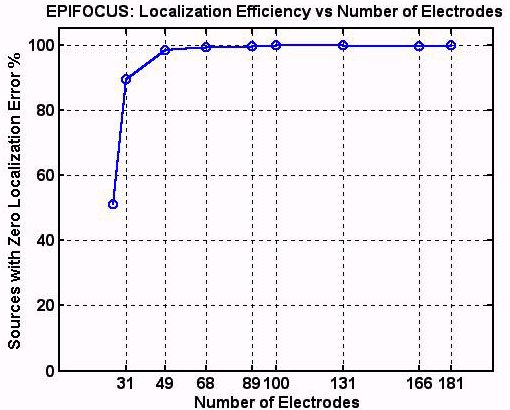
Figure 2. Number of sources with zero
localization error vs Number of electrodes for EPIFOCUS.
Note that a perfect localization (100%) can be already reached with a
relatively low number of electrodes (100). Electrode configurations on
this order are becoming a standard procedure in most of the research
labs.
3.2. Computer Generated Data with Noise
This section cannot include a comparative study of all the solutions
considered before due to a lack of data describing the behavior of these
solutions in the presence of noise. For that reason, we analyze the noisy
data only with the EPIFOCUS. As described before, the noisy data is
obtained by adding to the noiseless data an uncorrelated noise vector
that can change from -15% to +15% the value at each electrode. Since the
EPIFOCUS is already a quasi solution, i.e., it does not explain the data,
we use the same matrix computed for the noise free data. The results are
illustrated in Fig. 3.
The upper plot of Fig. 3 shows the empirical probability distribution
and the empirical density function for the source localization error.
Around 94% of the sources are still retrieved with zero localization
error and the maximum error is at maximum only 2 grid units. The second
entry depicts the average localization error that remains very close to
zero for all eccentricity values.
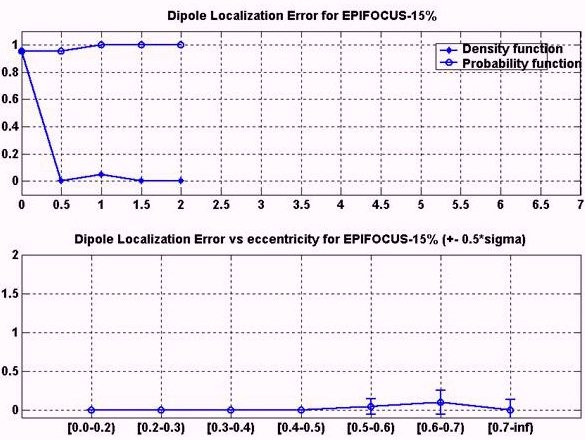
Figure 3. Dipole localization error (DLE) for
EPIFOCUS with noisy data. Upper: Probability and density function of the
DLE. Lower: Average localization error as a function of the source
eccentricity.
3.3. Analysis of Experimental Data
For the analysis of experimental data we consider realistic head
models derived from the anatomical MRI of each subject. After
segmentation of the anatomical images, a set of solution points belonging
to the 3D gray matter distribution is selected. The selected points
correspond to an irregular grid of points with distance between 4 to 6
mm. The SMAC method described in Spinelli et al. [Spinelli et al., 2000]
is used to locate the electrodes and compute the lead field. With this
lead field that summarize all the electrical and anatomical information
of the subject we compute the EPIFOCUS inverse as described in the
Appendix.
In Lantz et al. [Lantz et al., 2001a], we assessed the sublobar
accuracy of EPIFOCUS analyzing the same data where dipolar models [Lantz
et al., 1996] and LORETA [Lantz et al., 1997] found no significant
differences for the four epileptic sources detected within the temporal
lobe. In another study that will be presented elsewhere [Michel et al.,
in preparation] we analyzed 16 patients with temporal and extratemporal
epilepsies. In latter study, we applied EPIFOCUS to increase the accuracy
of the localization for those maps where LAURA solution provided a clear
evidence of a dominant (concentrated) source. EPIFOCUS results were never
in contradiction with the available additional independent information,
that is, for the case of visible lesions on the MRI the located source
was always within or in the vicinity of the lesion (tumor). For the
operated patients, the source was always within the resected area and for
all patients where intracanial electrodes were available, the recordings
confirmed the source localization results. The following examples discuss
the application of EPIFOCUS to two different epilepsy cases: an occipital
epilepsy and a temporal lobe epilepsy.
Note that in the following figures, the extent of the activated area
is strongly influenced by the simple neighbor interpolation law used to
overlay the discrete solution space on the anatomical MRI.
a) Occipital Epilepsy
From a methodological (not clinical) point of view this is a
really simple case for the inverse solution. According to the MRI, this
patient presented a clear lesion on the parieto-occipital region. For the
inverse solutions we considered averaged spikes measured on 125 surface
electrodes. The results of EPIFOCUS and the Weighted Minimum Norm (WMN)
are presented in Fig. 4. Although both solutions coincide in detecting a
clear occipital maximum they slightly differ in the lateralization of it.
Probably influenced by the noise, the WMN solution shows a maximum at the
left tip of the occipital lobe that extends also to the right. In
contrast, EPIFOCUSS shows a clear left occipital maxima nearby the MRI
lesion, which is not as superficial as the WMN maxima. The fact that the
WMN located the focus closer to the brain border than EPIFOCUS coincides
with the simulation result of the previous Section. In spite of this,
both inverse solutions are within the resected region and the patient is
seizure free.
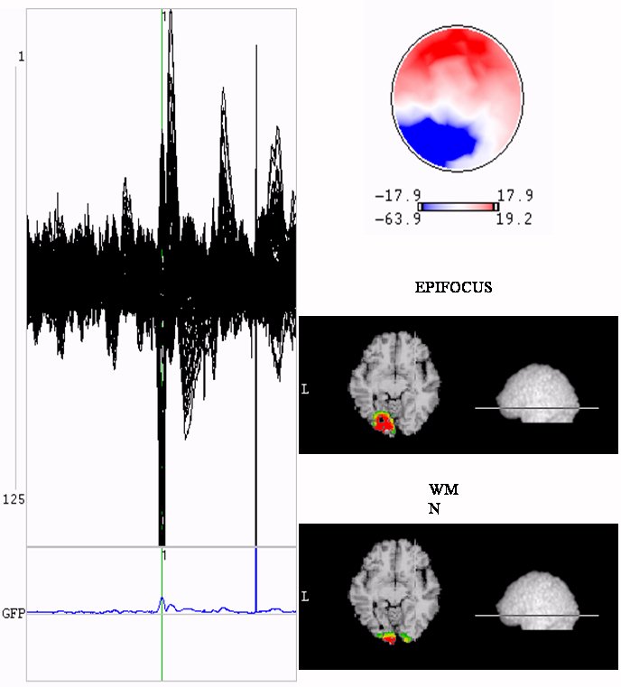
Figure 4. Occipital Epilepsy. Analysis of
averaged spikes on 125 electrodes without preprocessing. The upper left
panel shows the superposition of the 125 time curves (black) and lower
left the global field power (blue). Green marker (1) designs the latency
under analysis. Right side depicts the potential map and the inverse
solutions obtained at the marked latency. Only the slice of the maximum
is presented.
b) Temporal Epilepsy
For this temporal lobe patient an invasive pre-surgical study was
carried out since no abnormalities were detected in the structural (MRI)
or metabolic images. The EEG study was carried out using 125 surface electrodes,
and one sub-dural grid (8x8 contacts) as well as 2 stripes (2x4 contacts
and 3x6 contacts) on the right temporal lobe. The intra-cranial data
revealed [Lantz et al., 2001b] the temporal propagation of the epileptic
discharge from the anterior to the posterior part of the left temporal
lobe. For the inverse solution analysis, a set of averaged spikes
measured over the 125 scalp sensors were considered. While in Lantz et
al. [Lantz et al., 2001b] we preprocessed the data (filtering,
segmentation and averaging of adjacent maps) before the application of
the WMN, here we describe the results of applying the inverse solutions
to the raw data resulting from spikes averaging.
Figure 5 shows the localization results obtained for both solutions.
The upper left part depicts the superposition of the 125 electrodes
waveforms resulting from the averaging process (black traces) and the
global field power (GFP) in blue. The three green markers (1, 2 and 3)
indicate approximately 3 maxima of the GFP corresponding to the latencies
where the frontal (1) to posterior (3) transition was detected from the
intracranial electrodes. The upper right part depicts the three potential
maps at the marker positions and the lower part presents the results of
the inverse solutions for the three latencies.
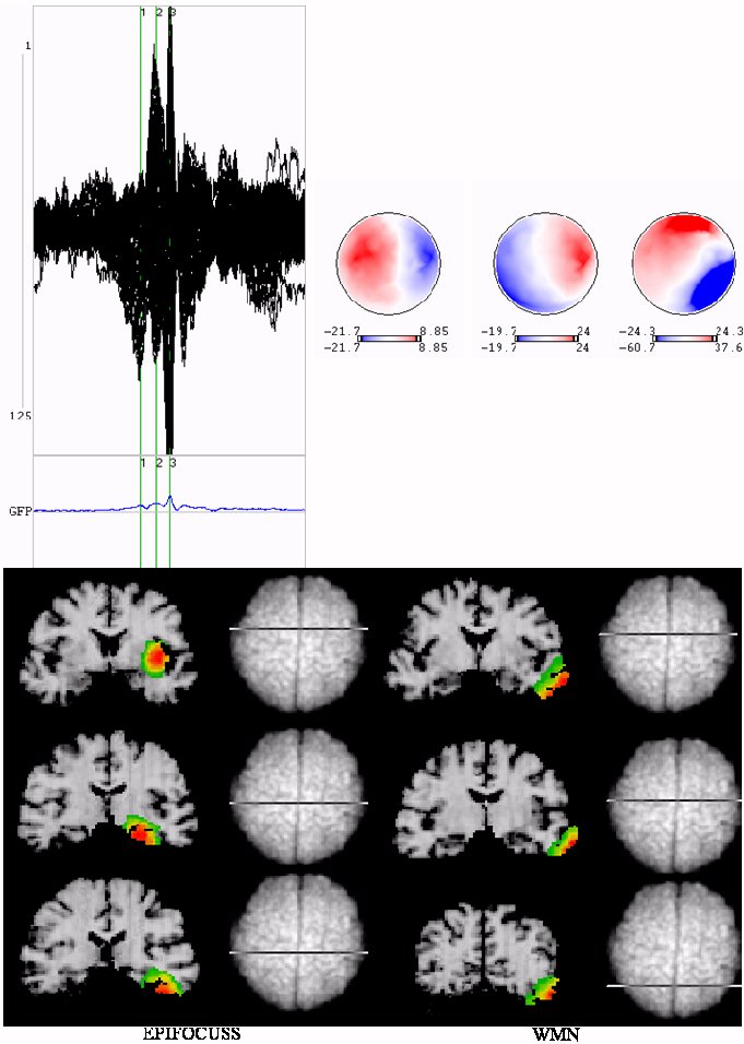
Figure 5. Right temporal lobe Epilepsy.
Analysis of averaged spikes on 125 electrodes without preprocessing. Upper
left: superposition of the 125 time curves (black) and global field power
(blue). Green markers (1, 2, 3) design the latencies where transfer was
observed from intracranial electrodes. Upper right: potential maps at the
3 marked latencies. Lower side: Results of the inverse solutions for the
three latencies. First row corresponds to first latency and so on.
EPIFOCUS solution is shown on the left and WMN on the right. On the MRI
images right is right.
Note that EPIFOCUS clearly identifies the propagation of the seizure
discharge (from the anterior to the posterior part of the temporal lobe)
coinciding with the intracranial measurements. While from the cortical
intracranial grid it is impossible to assess whether the source was at
the brain cortex or in a deeper non cortical region, the simulation
results induce us to trust the source depth suggested by EPIFOCUS.
EPIFOCUS provided consistent localization results for sources everywhere
in the brain (deep and cortical) in both noisy and noise free simulations.
As we obtained already [Lantz et al., 2001b], the reconstruction provided
by the WMN is very superficial and seems to be more sensitive to noisy
the data, e.g., the reconstruction for the third latency is too posterior
(see Fig. 5, lower right, third row). After the (standard en bloc)
resection of the right temporal lobe the patient is seizure free.
4. Conclusions
In this paper we presented a comparative study about the performance
of the Minimum Norm (MN), the Weighted Mimimum Norm (WMN), the Minimum Laplacian
(LORETA), LAURA and EPIFOCUS, in the localization of single sources
without noise.
The two new solutions, LAURA and EPIFOCUS, produced the best results
in terms of the number of sources with zero localization error, maximum
localization error, and average localization error as a function of the
source eccentricity. LAURA (32 %) increased by 12 % the number of sources
with zero localization error with respect to LORETA (20 %). EPIFOCUS
yielded 95 % of sources with zero localization error. The new methods
reduce the maximum error from 5.48 (MN), 5.20 (WMN) and 3.16 (LORETA)
down to 2.45 (LAURA) and finally to 1 (EPIFOCUS). The average error of
LAURA is, except for one interval, better than MN, WMN and LORETA. The
average error of EPIFOCUS is very close to zero for all eccentricity
values.
The study of the performance of EPIFOCUS as a function of the number
of electrodes shows for the first time that it is possible to obtain
perfect localization (100 %) with a relatively low number of electrodes
(100 or more). Furthermore, the results of EPIFOCUS for noisy data, where
the maximum error is not bigger than 2 grid units and the average error
remains very close to zero, illustrate the robustness of this method. The
robustness of this method to noise obeys to the fact that it is a
quasi-solution, i.e., the data are not totally explained. The resulting
effect is similar to the one produced by regularization procedures that
attemp to increase the localization quality even if the predicted data
differs from the measurements.
In summary, the behavior of the EPIFOCUS with both synthetic noiseless
and noisy data and experimental data indicate that we have at our
disposal an accurate and computationally efficient tool for the
localization of concentrated sources (not necessarily dipolar). As shown
here, this is immediately applicable to the analysis of epileptic data
with the advantage over single dipole models of being a method easy to
implement in scattered solution spaces as the ones arising from
segmentation of the individual subject MRI. The availability of high
accurate localization methods such as the EPIFOCUS may become important
in the future, for instance for identifying cases where
amygdalo-hippocampectomy or other limited temporal lobe resections may replace
the standard en bloc resections.
The comparative results described in this paper allow extracting some
theoretical conclusions useful for the design and implementation of
linear inverse solutions. That EPIFOCUS localizes all sources with zero
dipole localization errors confirms that the dependence of the inverse
matrix on the a priori information allows for the controlled adjustment
of the columns of the resolution matrix, that is, the accurate retrieval
of single sources, theoretically predicted in Grave and Gonzalez [Grave
and Gonzalez , 1998]. This means that it is possible to design linear
solutions with quasi-optimal performance in the determination of the
position of single sources, i.e., the columns of the resolution matrix
can be adjusted at will to obtain quasi-optimal impulse responses [Grave
and Gonzalez, 1998] and thus, very low or even zero dipole localization
errors.
The interpretable neurophysiological results obtained in a large
variety of experimental event related data [Michel et al., 2001] support
the choice of LAURA when the assumption of a single dominant source is
not expected to hold. Still the constraints used in LAURA obey physically
driven laws more likely to manifest with experimental data than with
mathematically generated source models such as the current dipole.
However, the results of this paper indicate that these physically driven
constraints are indeed a reasonable choice to deal with dipolar sources
in the absence of any a priori information.
An additional theoretical conclusion derived from these results is
that a lower dipole localization is neither a sufficient nor a necessary
condition for the performance of a linear inverse solution. Moreover,
EPIFOCUS and LAURA are particular cases of the WROP family [Grave et al.,
1998] which demonstrate that the Weighted Resolution Optimization is an
approach able to produce methods with poor single dipole localization
properties such as the column Weighted Minimum Norm (WMN) but also
optimal single source trackers as LAURA and EPIFOCUS.
While the analysis presented here considers only the electrical case,
there is no theoretical reasons to expect different results for the
magnetic case.
Acknowledgements
Thanks to Mr. Denis Brunet for expertise in designing the analysis
software and Drs Micah Murray, Goran Lantz and Christoph Michel for their
comments on previous versions of this manuscript. Research supported by
the Programme commun de recherche en genie biomedicale 1999-2002 and
the Swiss National Foundation grant 3100-065232.01.
References
Ary JP, Klein SA and Fender DH. Location of sources of evoked scalp
potentials: corrections for skull and scalp thickness. IEEE
Transactions on Biomedical Engineering, 28:447-452, 1981.
Berg P and Scherg M. A fast method for forward computation of
multiple-shell spherical head models. Electroencephalography and
Clinical Neurophysiology, 90: 58-64, 1994.
Fuchs M, Wagner M, Köhler T, Wischmann H-A. Linear and nonlinear
current density reconstructions. Journal of Clinical
Neurophysiololy, 16:267-95, 1999.
Golberg MA, (Ed.). Solution Methods for Integral Equations, Plenum
Press, New York. 1978.
Goronidnitsky IF, Rao BD. Spatial signal reconstruction from limited
data using FOCUS: a reweighted minimum norm algorithm. IEEE
Transactions on Signal Processing, 45 (3)" 1-16, 1997.
Grave de Peralta 1-14 R, Hauk O, Gonzalez Andino S, Vogt H and
Michel CM. Linear inverse solutions with optimal resolution kernels
applied to the electromagnetic tomography. Human Brain Mapping,
5:454-467, 1997.
Grave de Peralta 1-14 R. Gonzalez Andino S and Lütkenhöner B.
Figures of merit to compare linear distributed inverse solutions. Brain
Topography, 9:117-124, 1996.
Grave de Peralta 1-14 R, Gonzalez Andino SL. Distributed source
models: Standard solutions and new developments. In: Analysis of
neurophysiological brain functioning. Uhl,C. (Ed.). Springer Verlag,
1999, pp. 176-201.
Grave de Peralta 1-14 R, Gonzalez Andino SL. A critical analysis
of linear inverse solutions. IEEE Transactions on Biomedical
Engineering, 4: 440-48, 1998.
Grave de Peralta 1-14 R, Gonzalez Andino SL, Morand S, Michel, CM,
Landis TM. Imaging the electrical activity of the brain: ELECTRA. Human
Brain Mapping, 9: 1-12, 2000.
Grave de Peralta 1-14, R. Linear Inverse solutions to the
Neuroelectromagnetic Inverse Problem. PhD. Thesis N0. 3042. Faculty of
Sciences. Geneva University. Geneva. Switzerland, 1998.
Grave de Peralta 1-14 R. Gonzalez, S.L. Discussing the
capabilities of laplacian minimization. Brain Topography,
13(2):97-104, 2000.
Grave de Peralta R, Gonzalez SL, Lantz G, Michel CM, Landis T.
Noninvasive localization of electromagnetic epileptic activity. I Method
descriptions and simulations. Brain Topography 2001. (In press)
Hämäläinen MS, Ilmoniemi RJ. Interpreting measured magnetic fields of
the brain: Estimates of current distributions. Technical Report
TKK-F-A559, Helsinski University of Technology, 1984.
Huiskamp G, van Oosterom A. The depolarization sequence of the human
heart surface computed from measured body surface potentials. IEEE
Transactions on Biomedical Engineering, 35:1047-58, 1988.
Lantz G, Holub M, Ryding E, Rosen I. Simultaneous intracranial and
extracranial recording of epileptiform activity in patients with drug
resistant partial epilepsy: patterns of conduction and results from
dipole reconstruction. Electroencephalography and Clinical
Neurophysiology, 99: 69-78, 1996.
Lantz G, Grave de Peralta R, Gonzalez S, Michel CM. Noninvasive
localization of electromagnetic epileptic activity. II. Demonstration of
sublobar accuracy in patients with simultaneous surface and depth
recordings. Brain Topography, 14:139-147, 2001a.
Lantz G, Spinelli L, Grave
de Peralta R, Seeck M, Michel CM. Tomographie électrique en
épilepsie : localisation de sources distribuées et comparaison avec
l'IRMf. Epileptic Disorders Vol 3, Special Issue No 1, 2001b.
Lawson CL, Hanson RJ. Solving least squares problems. Prentice Hall,
Inc., Englewood Cliffs, New Jersey, 1974.
Menke W. Geophysical data analysis: Discrete inverse theory. Academic
Press, San Diego, 1989.
Messinger-Rapport BJ, Rudy Y. Regularization of the inverse problem in
electrocardiography: a model study. Mathematical Biosciences,
89:79-118, 1988.
Michel CM, Thut G, Morand S, Khateb A, Pegna AL, Grave de Peralta R,
Gonzalez SL, Seeck M, Landis T. Electric source imaging of human brain
functions. Brain Research Reviews, 2001. (In press)
Moore E H. Bull Amer Math Soc, 26: 394-395, 1920.
Philips DL. A technique for the numerical solution of certain integral
equations of the first kind. Journal of the Association for Computing
Machinery, 9: 84-97, 1962.
Penrose R. A generalized inverse for matrices: Proc.Cambridge
Philos.Soc., 51: 406-413, 1955a.
Penrose R. On best approximation solutions of linear matrix equations:
Proc.Cambridge Philos.Soc., 52, 17-19, 1955b.
Pascual Marqui RD, Michel CM, Lehmann D. Low resolution
electromagnetic tomography: a new method for localizing electrical activity
in the brain. International journal of psychophysiology, 18:
49-65, 1995.
Rao CR, Mitra SK. Generalized inverse of matrices and its
applications. John Wiley & Sons, Inc., New York. 1971.
Ripley BD. Spatial Statistics, Wiley, New York, 1981.
Spinelli L, Lantz G, Gonzalez SL, Michel CM. Anatomically constrained
spherical head model for EEG source localization. Brain Topography,
13, 115-125, 2000.
Stok CJ. The inverse problem in EEG and MEG with application to visual
evoked responses. CIP Gegevens Koninklijke Biblioteek, The Hague, 1986.
Tihonov AN, Arsenin VY. Solutions of ill-posed problems. Wiley, New
York. 1997.
van Oosterom, A. History and evolution of methods for solving the
inverse problem. Journal of Clinical Neurophysiology, 8:371-380,
1992.
Wagner M, Fuchs M, Wischmann HA, Drenckhahn R, Köhler T. Smooth
reconstructions of cortical sources from EEG and MEG recordings. Neuroimage,
3:168, 1996.
Wahba, G. Spline models for observational data. Society for Industrial
and applied mathematics. Philadelphia, Pennsylvania, 1990.
APPENDIX
For the researcher interested in testing concrete inverse solutions,
we provide here all the mathematical details needed for their
implementation.
LAURA (Local AUtoRegressive Average) solution
In Grave et al. [Grave et al., 2000] we presented a new source model
constrained by the physical properties of the generators of the
electrical activity. This alternative source model (ELECTRA) allows the
restatement of the bioelectric inverse problem in three mathematically equivalent
ways. One of them transformed the original problem associated to the
estimation of the current density vector (3D vector field) into the
determination of the potential in depth (scalar field). Although the
formulations described in ELECTRA are more restrictive, the solution is
still non-unique, i.e., infinitely many solutions still exist. However,
the physical properties of the unknown field (potential in depth) can
also be considered to soundly pick up one of these solutions. The
resulting solution strategy coined LAURA takes into account the physical
features in the following way:
a) Since the potential in depth is scarcely determined by the external
potential measurements, the resulting inverse problem is highly
underdetermined. In other words, EEG measurements are not sufficient to
fully determine the activity at all brain locations. Consequently, the
electrical activity at each point can be expressed as a combination of
the information supplied by the data and the local neighbors.
b) According to elementary potential theory, the Newtonian potential
is a function of the inverse of the distance, electric potentials decays
as a function of the square distance and the electric fields decays with
the third power of the inverse distance. To include both aspects we
express the activity at each point as a function of the neighbors by
means of a local autoregressive estimator [Ripley, 1981] with
coefficients that depend on the distance to the target point, that is,
| |
 |
(A-1) |
This
equation express the unknown function value at the i-th point as a
weighted sum of the unknown function values at the neighborhood as
proposed by Grave and Gonzalez [Grave and Gonzalez, 1999]. Since the sum
of the weigths is one, equation A-1 describes a consistent local average.
The maximum number of neighboors is N=26 for a 3D vicinity and Ni
is the actual number of neighboors of point i. A neighboorhood is defined
by the hexaedron centered at the target point. Such selection allows for
the consideration of solution spaces derived from anatomical images where
the intergrid distances might differ in the three coordinate axes. For
all solution points we use the same exponent ei=1 or 2 or 3 to
express the dependence with the distance.
The factor Ni/N allows for the correct estimation of the
constant function while incorporating into the formulation the fact that
no primary sources exist outside the brain and consequently function
values are zero outside the brain borders.
Multiplying both sides by an arbiratry factor wi>0 and
substracting both sides of (A-1) and reorganizing we can obtain a new
scalar field that defines implicitely a regularization operator [Grave
and Gonzalez, 1999]:
| |
 |
(A-2) |
In other words, LAURAs approach minimizes the norm of the field g, which
has components that are "spatially more independent" than those
of f. One element of g (nearly) zero implies that the
corresponding element of f, is (almost) fully predicted from its
neighbors (A-1) and not by the data.
Considering the discrete version of the problem:
| |
 |
(A-3) |
Where d stands for the data measured on ns sensors, J is
the discretization of the unknown function on np solution points and
vector n represents the additive noise present in the data. The
solution is obtained by solving the following variational problem for the
unknown Np-vector J
| |
 |
(A-4) |
The regularization operator reads:
| |
 |
(A-5) |
According to (A-2), the diagonal element of
the i-th row of A is:
| |
 |
(A-6) |
Where Vi
stands for the vicinity of the i-th solution point and dki
is the distance from the k-th neighbor to the target point i. The
off-diagonal elements are zero except for kÌVi
where the value is given by:
| |
 |
(A-7) |
When using the source model
of ELECTRA (potential in depth), unless we have some additional
information we set the diagonal matrix W to the identity and ei=2.
For the estimation of the current
density vector (vector field with 3 components), one can apply previous
operator by components . In this case, the regularization operator reads:
| |
 |
(A-9) |
where the symbol Ä represents the kronecker product of
matrices [Rao and Mitra, 1971], and the elements of the diagonal matrix W
are selected as the mean of the norm of the 3 columns of the lead field
matrix associated with point i. This new weighting strategy increased
significantly the localization capabilities of LAURA. While higher
exponent values, e.g. ei=11, can increase the number of
sources perfectly localized up to 50 %, in Table 1 we consider only
exponent values derived from potential theory, that is, ei=1,2
and3.
With previous definitions
the products M=WA (scalar field) and M=WAÄI3 (3D vector field)
are invertible and the inverse matrix can be computed as:
| |
 |
(A-10) |
For an efficient
numerical implementation of equation A-10 consider the following
elements:
a) According to the basic
kronecker product properties [Rao and Mitra, 1971] only matrix WAtAW
has to be inverted.
b) Since all the matrices to be
inverted are symmetric and positive definite then, compute only the upper
triangles and use Cholesky algorithm for the inversion.
c) Note that the product (RRtÄI3 )Lt, where
R is a Cholesky (triangular) factor of (WAtAW)-1,
can be done without the explicit computation of the Kronecker product.
EPIFOCUS
Assuming that the data is generated by a
single source and accepting (as is the case for all regularization algorithms)
that the solution will not perfectly explain the data, we can obtain an
inverse matrix highly sensitive to focal sources. The intuitive idea
behind this method is to change the original problem to a new space (or
variable) such that the projection over each location has an increased
contrast power. For the mathematical implementation, note that the lead
field has the following structure:
| |
 |
(A-11) |
where each block Li
is formed by ns rows and 3 columns associated with the potential
generated by the three orthogonal unitary dipoles that can be placed
at the i-th solution point. The two following steps produce the
desired inverse matrix:
a) Change of variable.
Compute the transformed lead field matrix T by normalizing each
column of L, i.e., T=L*W, where W is a diagonal
matrix with elements equal to the inverse of the norm of the columns of L.
Matrix T has the same structure of L, i.e.,
| |
 |
(A-12) |
b) Computing the local
projectors. To obtain the inverse G, compute the Moore-Penrose pseudo
inverse [Rao and Mitra, 1971] of each block and arrange them in the
following way:
| |
 |
(A-13) |
The product of this
inverse matrix G with the recorded data yields an estimator of the
weighted current source density. The plot of the modulus of this estimate
for each solution point can be interpreted (up to a scaling factor) as
the probability of a focal source at that point. The column weighting
used in the change of variable (step a), is essential for the
localization features of EPIFOCUS and distinguishes it from other
projectors used so far. While this weighting corresponds to the widely
used column Weighted Minimum Norm [Lawson and Hanson,1974], it has never
been applied to the case of projectors as in Equation (A-13).
| 
 Home
Current Issue
Table of Contents
Home
Current Issue
Table of Contents
