1. Introduction

While there is hardly any lack of electrocardiographic or magnetocardiographic data, detailed data on the anatomy and physiology of the conduction system or cellular interactions in the myocardium are scarce [Durrer et al., 1979]. We may even have access to high-quality recorded data on the endocardial and epicardial potentials during cardiac activation [Gepstein et al., 1997], but we are left to guess how exactly the propagation through the myocardium takes place. However, a ventricular model that produces a correct normal activation sequence is a prerequisite for simulating pathological conditions, such as ischemia, infarction or ventricular arrhythmias [Berenfeld and Jalife, 1998]. Therefore, a comprehensive model should feature an anatomically accurate geometry, intramural fibrous structure, and a conduction system, and the action potential of a single cell should be modeled realistically. As if there were not enough difficulty in obtaining accurate data to base the modeling on, implementing the models themselves is a challenge.

First idealized models describing the normal activation sequence in the human heart were reported over two decades ago [Ritsema van Eck, 1972; Miller and Geselowitz, 1978]. Mainly due to computational limitations, the models did not include myocardial anisotropy or physiological propagation. On the basis of anisotropic bidomain theory [Colli Franzone et al., 1983] and cellular automata theory [Toffoli et al., 1987], development of more realistic whole-heart models has become feasible [Leon and Horáček, 1991]. In this paper, we concentrate on the modeling of the interacting cellular elements and the bidomain equations, implementation of the conduction system and the computation of extracardiac electromagnetic fields. As our model of the action potential is still primitive, we are also limiting ourselves here to discussing the ventricular depolarization.

 

 

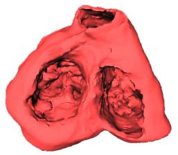
Figure 1. Left: Fiber arrangement on an yz-cross section approximately in the middle of the ventricles. The principal fiber directions are marked with arrows. The angles, measured from the local tangent vector at each element, rotate from about -50 degrees on the endocardium to about +45 degrees on the epicardium. Right: Three-dimensional presentation of the ventricles as seen from the base of the heart.

2. Methods

2.1. Anisotropic Propagation Model and the Cellular Elements

The propagation model consists of 2.000.000 excitable elements comprising the conduction system and the myocardium and 8.000.000 non-excitable elements making up the intra- and extracardiac volumes. The elements are located on a cubic lattice with 0.5-mm spacing [Hren et al., 1998]. The geometry was reconstructed from 1-mm sections of the human heart [Ritsema van Eck, 1972]. The assignment of the principal fiber direction was performed separately for left-ventricular, right-ventricular and papillary-muscle cells, with the fiber direction rotating from endocardium to epicardium [Streeter, 1979]. Fig. 1 illustrates the amount of anatomical detail that was included in the model.

Our hybrid model of the anisotropic myocardium describes the subthreshold behaviour of the elements according to the bidomain theory [Colli Franzone et al., 1983], while in the suprathreshold region the elements behave as cellular automata [Toffoli and Margolus, 1987]. Each element is assigned a specific type and a vector of local fiber direction based on anatomical data [Leon and Horacek, 1991; Taccardi et al., 1994]. Each element can be in one of four macrostates, corresponding to different phases of an action potential: resting, excitatory, absolute refractory, or relative refractory. During simulation, elements undergo a series of macrostate transitions, which have been described in detail in [Nenonen et al., 1991]. The subthreshold transmembrane potential, v_m is calculated from the generalized cable equation, derived from the anisotropic bidomain theory [Colli Franzone et al., 1983]:

  

(1)

Here we assume that the assumption of equal anisotropy ratios is valid [Leon and Horacek, 1991; Nenonen et al., 1991]. In Eq. 1, c_m is the specific membrane capacitance, D_i is the intracellular conductivity tensor, and i_ion and i_app are ionic and applied currents, respectively. Above a threshold value, the cell enters the absolute refractory state and v_m is estimated from a predefined function consisting of an upshoot part and a logarithmic plateau phase [Nenonen et al., 1991]. Physiological parameters like the conductivities and the specific membrane capacitance for the model are adopted from literature [Colli Franzone et al., 1983; Roth, 1991].

The correct discretization of Eq. 1 is crucial for a directionally unbiased activation. Since the cell size is reasonably large compared to the dimensions of the ventricular structures, the estimation of the divergence of the current density is done in a 3x3 cube of cells. Now, using traditional differentiation stencils that misemphasize the diagonal directions can, e.g., turn the activation in the direction of the coordinate axes. Here, a method similar to the “natural neighbors” method [Braun and Sambridge, 1995] can be used to alleviate the problem.

2.2. Extracardiac Field Calculation

In the forward computations, the ventricles are assumed to be embedded in a torso-shaped piecewise homogeneous volume conductor, including the lungs and the intracardiac blood masses. The infinite medium potential f_o in the extracardiac region is determined from the discretized equation

(2)

where the integrals are evaluated over the ventricular volume, v_m is as in Eq. 1, a is the local direction of the fiber axis, s is the extracellular conductivity (s = 2.0 mS/cm), s₁ is the transverse conductivity (s₁ = 0.5 mS/cm) and s₂ is the difference between the axial and transverse conductivity (s₂ = 1.5 mS/cm) [Nenonen et al., 1991]. The first term of the potential in Eq. 2 represents the contribution of the isotropic component and the second term accounts for the anisotropic properties of the cardiac tissue. The extracardiac magnetic field H_o is evaluated from a corresponding equation,

  

(3)

To compute the body surface potential and magnetic field in the inhomogeneous torso, a "fast forward solution" is used [Nenonen et al., 1991]:

  

(4)

In Eq. 4, W is a geometry matrix consisting of the solid angles subtended by a surface element at each node, and A is another (vector-value) geometry matrix taking into account the influence of the conductivity change surfaces on the magnetic field (for details, see [Nenonen et al., 1991b]). The anisotropy of the volume conductor can be estimated by the thorax extension method [Lorange and Gulrajani, 1993].

When the Eqs. 2 and 3 are discretized and subsequently the integration (or summation) is carried out, special care has to be taken that the elementary current sources do not contribute to the fields multiple times. If one aims at a good approximation of the elementary sources, a differentiation stencil of 2x2 or 3x3 elements needs to be used. However, since the integrand is vector-valued, any contribution from the diagonal element pairs easily misweights the elementary dipoles. Some error is also always present due to the fact that the fiber direction used for estimating the (finite-size) dipole at a certain location is computed from the starting point of the dipole, not the center.

2.3. Conduction System

The organization of the conduction system was created by using information available from textbooks on human anatomy and other literature on the topic [Berenfeld and Jalife, 1998; Demoulin and Kulbertus, 1982; Durrer et al., 1979; Tawara, 1906]. In anatomical studies, the left bundle branch has been found to be a sheet-like structure that covers a large portion of the interventricular septum. The fascicles in the branch are highly interconnected. The anterior rim of the left bundle travels towards the left anterior papillary muscle, while the posterior rim is oriented toward the left posterior papillary muscle. The right bundle branch usually begins from the most distal part of the His bundle. It courses subendocardially and intramyocardially towards the right anterior papillary muscle. At the papillary muscle, it divides into fascicles that continue as the right Purkinje network leading the activation to the posterior papillary muscle and the right ventricular free wall. The His bundle continues on both sides as the Purkinje network that contains the Purkinje-myocardial junction (PMJ) sites. On the right, the most prominent feature of the conduction system is the single bundle that carries the activation from the septum to the free wall and the papillary muscles along the moderator band. On the left, there are three major areas of activation: the septum and the inferior and superior free wall.

Figure 2. The geometry of the conduction system observed from different angles. The right branch of the His bundle (not shown) connects the topmost nodes of the left and right conduction system. In the right ventricle, the moderator band contains the conduction system activating the RV free wall and the papillary muscles. The RV free wall (a) and septal (b) views show the right conduction system, consisting of one main bundle with several smaller branches.The views of LV septum (c) and LV free wall (d) show the more complicated structure of the left conduction system. Notice the fan-like structure of the septal conduction system in (c), and the vertical spiral gap in the conduction system in (d). The PMJs are shown as light green spheres.

The gross geometry of the conduction system is shown in Fig. 2. To obtain correct electromagnetic fields on the body surface, the conduction system has to be carefully tuned. The right balance between the activation times in the left and the right ventricle is necessary to create a correct 12-lead ECG and VCG. On the other hand, to obtain a ventricular activation sequence corresponding to measured data [Durrer et al., 1979], the correct location and number of the Purkinje-myocardial junction sites is crucial. In the course of tuning, it often happens that these two requirements cannot be fulfilled by the same conduction system model. Therefore, the tuning of the model was performed sequentially for the isochrones of Durrer, the body surface potential and magnetocardiographic maps and finally for the 12-lead ECG and the vectorcardiogram.

3. Results

3.1. Propagation in the 3D Ventricles - Isochrones

The simulated activation sequence resulting from the activation of the conduction system is shown in Fig. 3. The ventricular activation starts in the left ventricular septum (layer 110), matched by a right ventricular septal activation 20 ms later (layers 70-90). Almost simultaneously with the RV septal activation, the inferior (in body coordinates) and anterior LV activation appear (layers 90-110). These are followed by the activation of the RV free wall (layers 90-130). The RV and LV breakthroughs take place at 30 ms and 45 ms, respectively. In the final stages of the QRS, activation propagates through the posterior LV free wall and the pulmonary conus. The result agrees well with isochrones obtained from an isolated human heart [Durrer et al., 1979]. Some minor differences can be seen in the activation of the right ventricle. However, based on high interindividual variability in Durrer's work and other literature sources describing the human ventricular activation [van Dam, 1976], the RV activation sequence seems to be somewhat unclear. Therefore, we trusted our model of the conduction system to be correct, since the electromagnetic fields produced by the activation were in agreement with our recordings. A three-dimensional view of the activation isochrones is shown in Fig. 4.

Figure 3. Simulated activation isochrones. The 20 layers are with a spacing of 10 mm, and correspond to those presented by Durrer et al. The isochrone spacing is 5 ms.

a)	b)
c)	d)

Figure 4. Three-dimensional views of the simulated isochrones. a) Anterolateral apical view of the right ventricle, b) oblique cross section across the ventricles c) posterolateral basal view of the left ventricle, d) a cross section showing the intramural activation isochrones in both ventricles.

3.2. Simulated BSPM and MCG Patterns

BSPMs were evaluated on the nodes of a triangulated torso model of an adult male, while the normal component of the cardiomagnetic field (MCG) was computed on a plane array in front of the chest. Fig. 4 shows simulated BSPM and MCG distributions during the QRS complex. In BSPM, the initial maximum resulting from left septal activation is anterior. Then the minimum on the back moves upward and travels over the right shoulder onto the right anterosuperior region, indicating apical activation and masking of the left septal activation by the corresponding right-septal activation. The area of positive potentials then drifts to the back. In the end, the activation propagates toward the pulmonary conus, reflected as a superior positive potential in BSPM. The sequence of MCG patterns essentially depicts the direction of the frontal ECG vector, i.e. the direction of activation in the plane of the frontal chest.

The mean body surface potential map series of healthy patients displays a similar time development as the simulated BSPM. What is noteworthy here again is the large interindividual variability, which is certainly understandable. The diversity of conduction systems is added to by the differences in body shape, the volume conductor properties and even the physiological state of the patient during the recording. For example, the initial maximum may well be located on the lower half of the chest, and the rotational movement may take place from right to left on the frontal chest, not diagonally. Against this, the simulated BSPM patterns seem acceptable.

Figure 5. Simulated BSPM distributions at 10 ms steps during the QRS complex. The read and blue areas denote, respectively, positive and negative values. At 50 ms, the positive area has moved to the back (not shown on the series).

Figure 6. Simulated MCG distributions at 10 ms steps during the QRS complex. The red areas denote positive values, where the magnetic flux enters the chest, while in blue areas the flux comes out of the chest.

3.3. Simulated Electrocardiograms and Vectorcardiograms

The “normal” 12-lead electrocardiogram is even more difficult to define than the normal BSPM, but some common features should anyway be present in the ECG to fulfill “normality”. The dominant features affecting all leads are – as can be seen from the BSPMs – that, in the beginning of the QRS complex, the left leg is positive and in the end, the activation propagates towards the back. This means that V1 and V2 should display a mainly negative morphology (activation away from the electrode) preceded by a small positive deflection. On the other hand, in the leads V4, V5, V6, I, II and aVF, positivity is the dominating feature. As can be seen, the simulated ECG fulfills these criteria reasonably well. However, the detailed morphology of the chest leads is somewhat incorrect, probably due to thorax modeling problems.

Figure 7. Simulated ECG leads and the vectorcardiographic loops. Top: ECG leads V2, V6, II and aVF. Bottom: the frontal, horizontal and sagittal VCG loops. The potential grid spacing is 0.5 mV and the time grid spacing (ECG) is 10 ms. Note how the frontal VCG loop is directed towards the left leg.

 

The normal vectorcardiogram (VCG) is characterized by a loop, whose average direction is to the left, down and slightly back. The frontal loop is very thin, and the sagittal and horizontal loops are somewhat wider. The sagittal and horizontal loops are clearly counter-clockwise. The frontal loop defines a clear “angle” that should be from –20^o to +110^o from the vertical axis pointing down. The simulated vectorcardiogram also follow this pattern well.

4. Discussion

Information from anatomical and electrophysiological studies on the conduction system are to some extent contradictory. The modelling is further complicated by the fact that anatomical information on the conduction system is old, and no digital data are available. Furthermore, few thorough works on activation sequences of the human heart exist.

Several details of the model algorithm are still under discussion in the scientific community. It is still somewhat unclear, whether simplifying the modelling of anisotropic properties by the use of equal anisotropy ratios affects the propagation significantly. The effect of thoracic and cardiac muscle anisotropies on the forward solution has also been discussed. However, more fundamental features like transmurally varying cell properties may mask the effects of anisotropy.

The activation sequence produced by our simulations was compared to the activation sequence measured from the isolated human heart. The simulated activation of the left ventricle matched very well the recorded one, when the cross sections are aligned. However, the data from Durrer et al. almost completely lacks right septal activation, which is necessary to produce correct ECG.

The simulated body surface potential pattern corresponds to our recorded BSPMs with the exception of two features: the initial positive area on the anterior chest moves slightly too quickly to the back and the late activation (positive) of the pulmonary conus is too strong on the anterior chest. Both these features may be attributed to inaccurate positioning of the ventricular model within the thorax. The magnetocardiographic maps are also consistent with recorded data. The general outline on the simulated 12-lead ECG is normal, and the vectorcardiogram is completely in the normal limits, the frontal angle being close to 60^o.

Acknowledgements

This research was partly financed by the Jenny and Antti Wihuri Foundation and the Emil Aaltonen Foundation. The first author also wishes to express his gratitude to Nokia Mobile Phones for supporting the work.

References