Principal Components Analysis:
An Old but Powerful Tool for ECG Analysis

Robert L. Lux

Nora Eccles Harrison Cardiovascular Research and Training Institute,
University of Utah, Salt Lake City, Utah USA

Correspondence: Robert L Lux, CVRTI, University of Utah, 95 South 2000 East, Salt Lake City, UT 84112-5000, USA.
E-mail: lux@cvrti.utah.edu, phone 801-587-9592, fax 801-581-3128

---

---

1.    Introduction

Principal components analysis (PCA), Karhunen-Loeve (KL) analysis, and factor analysis are related methods from a class of powerful analytic techniques that have proven to be extremely useful in the study of physical and biological systems and phenomena. These techniques offer means to dissect complex, multidimensional, and interdependent data sets into fundamental, independent building blocks that facilitate the characterization, understanding and explanation of the systems and phenomena from which they were derived. These techniques have been applied to electrocardiographic signals for over four decades and continue to provide insight into data structure as well as to facilitate identification of abnormal cardiac electrical behavior. ^1-7

The basis of these statistical methods may best be understood by relating them to their deterministic counterparts, the orthogonal series or expansions of mathematics. The classical Fourier series is one such expansion which is familiar to any student of mathematics, physics or engineering: given an arbitrary periodic waveform or signal, it is possible to mathematically characterize that waveform with an infinite sum of sine waves having amplitudes, frequencies and phases that are easily calculated. Importantly, each of these sine waves (the basis functions) is orthogonal to (independent of) any of the other sine waves, over integral numbers of periods of the waveform. The sine waves are the basis functions that describe how to reconstruct the original periodic waveform. The same endpoint can be achieved using a variety of other orthogonal series, e.g., Tchebychev polynomials, Legendre polynomials, etc., each of which has characteristics that may be appropriate for particular applications.

In contrast to these deterministic approaches, the need to characterize or represent signals or data measured from complex biological or physical processes led to the development of the statistical methods of PCA, KL and factor analysis. In place of mathematical functions, the basis functions of these methods are derived directly from the data themselves. This results in efficient representation, meaning that the accurate representation can be achieved with fewer basis functions than any other strategy. In addition to use of these techniques for representation, they provide means to compress data by minimizing redundancy, filter noisy data, and to define feature subspaces efficient for multi-class, multivariate discrimination.

2.    Methods

Derivation of the Eigenvalue Equation. We will start by considering a random vector, x, of dimension N that could represent samples of a waveform, or a one, two or three dimensional distribution of vectors, or some other random process. What we would like to do is to represent that random vector by an expansion of the type:

                                                            where                                                             (1)

where { f} is a set of yet to be determined orthogonal (orthonormal) vectors of dimension N, e.g.,

                                                                                                                                                          (2)

Since there is little to be gained by representing an N dimensional vector by a linear combination of N independent vectors, and since there is often redundancy in data, one might be able to represent x using M<N vectors with an acceptable error:

                                                                                                                                                          (3)

with an error of . Using least mean squared error analysis, one may show that the mean squared error, can be minimized by constraining the expansion coefficients {a} to be uncorrelated, i.e.

                                                          for I, j=1,2,….M                                                           (4)

where E is the expectation operator and l is a constant. Substituting Eq. 1 into 4, one obtains:

                                                                                                           (5)

where K is the covariance matrix of x. Since the ³ are orthogonal, a solution to Eq. 5 yields the classic eigenvalue equation:

                                                                                                                                                         (6)

the solutions for which are the eigenvectors {f} and eigenvalues {l} of the covariance matrix K of the random vector x. The power of this representation becomes clear: the basis functions of the expansion are derived from the statistical characteristics of the vector x itself and the eigenvalues of the covariance matrix reflect the importance of each respective eigenvector in explaining the distribution of the data. We say that the vector x is represented by the set of coefficients ³ in the sense that they are equivalent since x can be recovered or reconstructed via Eq. 1. Importantly, the eigenvalues and associated eigenvectors are normally calculated in the order of their importance (eigenvalue magnitude) and, in general, fall off exponentially. For most physical and biological systems, there is considerable redundancy in measured data, thus allowing for the possibility of representation using a small number of eigenvectors.

Geometric Interpretation of Eigenvectors and Eigenvalues. Perhaps the simplest example to help explain the meaning of eigenvectors and eigenvalues is to envision a 2D or 3D space with a scatter of points (vectors) in that measurement space of the two or three variables. In fact, the eigenvectors of the estimated covariance matrix fall along the dominant directions of point spread and are also orthogonal. The eigenvalues associated with each eigenvector are the variances of point spread along those eigenvectors. Hence, the eigen space is an equivalent coordinate space having the advantage that the coordinates or axes are aligned with the data and provide a means for knowing the importance of each axis for characterizing the data.

Redundancy reduction. Perhaps the most common use of these techniques is their application to data compression. For the case in which there is excessive redundancy in the data, M<<N basis functions may explain a high percentage of the data energy (variance). Returning to the point scatter example above, such data need only a few dimensions of the space to adequately characterize them. For example if the point scatter in 3D space falls mainly in one plane (2D) the eigenvectors define the coordinate axes of that plane and thus we need only 2 measurements to characterize the data points instead of 3.

Filtering, noise immunity. Another application of these techniques is filtering. Eigenvectors are robust descriptors of the data that they represent, but they are equally poor at representing noise or data that on average are not observed with high probability, i.e., waveforms or patterns that are not used in the construction of the covariance matrix. As such, the representation and then reconstruction, by forward and reverse application of Eq. 3 yields a filtered version of the original data that accurately characterizes those components of the signal that are explained by the eigenvectors, the example above helps to visualize this. Basically, noise creates outliers in data sets, and in a scattergram, an outlier falls outside the “usual” scatter of a defined group. When represented using a small number of space coordinates, only the relevant (most important) features of the data are retained.

Feature extraction and classification. A powerful use of these techniques relates to the need to classify data into one or more groups, the so-called multi-variate, multi-class discrimination problem. These representation methods provide a powerful means to determine which aspects of data sets are important in delineating multidimensional feature spaces for purposes of automatically classifying data into pre-determined groups. The eigenvectors determined from intra- and inter-class data provide important means to define features common to each class as well as features that best discriminate between classes. Although this topic is beyond the scope of this brief paper, the concepts are simple. Given multiple classes, each with point scatters in N dimensional space, one can envision the projection of each onto a subspace (plane) efficient for its respective class. The projections of point scatter from other classes will fall outside (probabilistically) the region occupied by the points that defined the subspace. In brief, original N dimensional measurement space maybe divided into subspaces optimal for differentiating class pairs.

Dissecting data into intrinsic components. The final application of these techniques is their use in understanding the intrinsic behavior of complex phenomena. Here, perhaps the best illustration is borrowed from the mathematics of differential equations that model physical systems. These equations, which arise from the characterization of electrical networks, control systems, or mechanical systems, have as their solutions, summation of natural modes of behavior. For example, the complex motion of coupled pendulums can be described by a summation of two sinusoidal functions, in which the frequencies reflect the individual resonant frequencies of each pendulum. The eigenvectors of the system are the individual sinusoids. Similarly, in the classic example of a system with damped oscillations, both exponential and sinusoidal behavior are observed, and in fact, the eigenvectors of the differential equation solution are an exponential and a sinusoid. In this, and many more examples, the eigenvectors of a system, whether physical or biological, statistical or deterministic, describe the fundamental behavior of that system. We shall illustrate this use of statistical representation theory in the example below.

3.    Results

As an example of the ability of these techniques to dissect out the fundamental behavior of data, consider the representation of the ST-T segment of the 12 lead electrocardiogram (ECG). We assembled digitized ECGs from normal subjects and patients with Long QT syndrome, for which the latter included patients with LQT1, LQT2 or LQT3 genotypes. Long QT syndrome is a disease in which the cardiac ion channels (potassium and sodium) are defective and as a consequence produce QT intervals that are abnormally long and can lead to arrhythmias and sudden death. We time-normalized all ST-T segments of leads I, II and V1-V6 between the J point and manually determined end of T and resampled each at 80 points. From the ensembles of 80 dimensional measurement vectors for each of the four classes, we estimated a covariance matrix from which we calculated the first ten eigenvectors and eigenvalues.

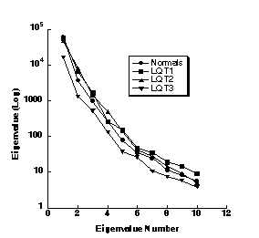
Figure 1. Eigenvalues of ST-T waveforms from normal subjects and patients with LQT1, LQT2 and LQT3 genotypes.

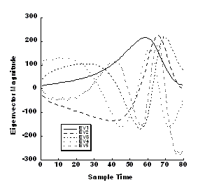
Figure 2. RMS normalized STT-T eigenvectors from normal subjects.

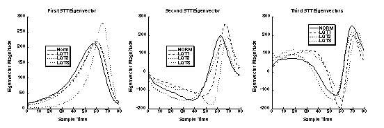
The data in Figure 1 show the first ten eigenvalues for each of the four classes. Clearly the data suggest that very few (3-4) independent waveforms are needed to accurately represent the original data. The data in Figure 2 show the first five root-mean-square (rms) normalized eigenvectors (waveforms) from the normal group of subjects. The “complexity” of these waveforms follow those observed naturally, e.g., the dominant T wave is a monophasic waveform, the next most important is a biphasic wave and so on. By summing these waveforms with appropriate weights (Eq. 3), the original waveforms can be reconstructed. Thus, each 80 sample ST-T waveform can be described by 4-5 numbers and the associated eigenvectors (waveforms). Finally, we show in Figure 3 the first, second and third eigenvectors for each of the four groups. Clearly they have features (morphologies) that are similar as would be expected from the fact that LQT patients have hearts that appear normal except for prolonged QT intervals and subtly abnormal T waves. In spite of the fact that QT interval was normalized out of this analysis, one can see that there are intrinsic differences in the ST-T waveform components determined for these groups. In particular, the LQT3 eigenvector shows a distinctly later and sharper peak in the dominant (first) eigenvector set. This is an observed feature of T waves in these patients. There is strong likelihood that these intrinsic features can be related to the abnormal sodium and potassium currents in these patients.

4.    Discussion and Conclusions

The methods of principal components analysis, the Karhunen-Loeve expansion and factor analysis are all similar, powerful techniques for using data to represent themselves. The power of the techniques relies in the extraction of independent features that can be used efficiently to characterize the same type of data. Thus in the above illustration, we used ST-T waveforms as the input data. The eigenvectors of the covariance matrix calculated from these data are themselves very much like the original data from which they were calculated. In fact they are the most efficient set of independent building blocks from which the original data could be reconstructed. As we discussed, these methods provide powerful, statistically robust means to apply data compression, noise reduction (filtering), estimation, feature extraction, and classification schemes to complex data sets.

Figure 3. First, second and third rms normalized ST-T eigenvectors for Normal subjects and patients with LQT1, LQT2 and LQT3 genotypes.

Acknowledgements

This work was supported in part by NIH grant HL 52338.

References

1. Scher A, Young A, Meredith W. Factor analysis of the electrocardiogram. Circ Res. 1960;8:519-525.

2. Horan LG, Flowers N, Brody D. Principal factor waveforms of the thoracic QRS complex. Circ Res. 1964;15:131-138.

3. Evans AK, Lux RL, Burgess MJ, Wyatt RF, Abildskov JA. Redundancy reduction for improved display and analysis of body surface potential maps. II. Temporal compression. Circ Res. 1981;49:197-203.

4. Lux RL, Evans AK, Burgess MJ, Wyatt RF, Abildskov JA. Redundancy reduction for improved display and analysis of body surface potential maps. I. Spatial compression. Circ Res. 1981;49:186-96.

5. Lux RL. Karhunen-Loeve representation of ECG data. J Electrocardiol. 1992;25 Suppl:195-8.

6. Mitchell LB, Hubley-Kozey CL, Smith ER, Wyse DG, Duff HJ, Gillis AM, Horacek BM. Electrocardiographic body surface mapping in patients with ventricular tachycardia. Assessment of utility in the identification of effective pharmacological therapy. Circulation. 1992;86:383-93.

7. Priori SG, Mortara DW, Napolitano C, Diehl L, Paganini V, Cantu F, Cantu G, Schwartz PJ. Evaluation of the spatial aspects of T-wave complexity in the long-QT syndrome. Circulation. 1997;96:3006-12.