It is well known that conventional EEG (i.e. 19 scalp electrodes disposed according to 10-20 International system) offers a high temporal resolution (milliseconds), but exhibits a low spatial resolution (about 6-9 cm) as an image of the cortical sources generating the potential. This is due to the different conductivities of cortex, dura mater, skull, and scalp (Gevins 1989; Nunez, 1995). The distortion of the recorded scalp potential distribution is further increased by the ears and eyeholes, which represent shunt paths for intra-cranial currents (Nunez, 1981, 1995). Another factor that affects the scalp potentials is the position and dynamics of electrical reference used during EEG recordings, which may filter out spatial components of the potential distribution over the scalp (Nunez, 1981). On the whole, the scalp potential distribution is a “blurred” copy of the original cortical potential distribution. Remarkably, the increase of spatial sampling (to 64 or 128) is not sufficient per se to enhance the spatial information content of scalp potential distribution (Gevins et al., 1999; Nunez, 1995).

Neural sources of EEG can be localized by making a priori hypothesis on their number and extension. When the EEG activity is mainly generated by a known number of cortical sources (i.e. short-latency evoked potentials), the location and strength of these sources can be reliably estimated by the dipole localization technique (Scherg and von Cramon, 1984). However, except for the processing of sensory inputs from the primary sensory cortical areas, the activity of multiple extended cortical sources has been reported in a variety of human tasks, i.e. simple movement planning and execution as well as complex memory tasks (Carlson et al., 1998). In these cases, the source activity could be estimated by using extended source models and spherical or realistic head volume conductor models in the context of linear inverse theory (Dale and Sereno, 1993; Pascual-Marqui et al. 1994; Grave de Peralta and Gonzales Andino 1998; Babiloni et al., 2000a; Dale et al., 2000). With this approach, thousands of equivalent current dipoles are used as a source model and realistic head models reconstructed from magnetic resonance images (MRIs) serve as a volume conductor (Meijs et al., 1993; Yvert et al. 1995). Regularized linear inverse solution attributes a strength value at each dipole of the source model from the scalp potential distribution.

The solution space (i.e. the set of all possible combinations of the cortical dipoles’ strengths) is generally reduced by using geometrical constraints, for instance by using cortical dipoles oriented according to the normal direction of the cortical surface. (Dale and Sereno, 1993). Constraints on the energy of the estimated cortical activity are decisive to reduce further the solution space (minimum-norm solution; Hamalainen and Ilmoniemi, 1984, Dale and Sereno, 1993). Recently, the solution space has been restricted by using information deriving from cerebral blood flow measures (Liu et al., 1998; Ahlfors et al., 1999; Babiloni et al., 2000b;  Dale et al., 2000; Liu, 2000). The rationale of such multimodal approach is that neural activity generating EEG potentials increases glucose and oxygen demands (Magistretti et al., 1999). This results in an increase in the local hemodynamic response that can be modeled by functional magnetic resonance images (fMRI; Grinvald et al., 1986; Puce et al., 1997). On the whole, such a correlation between electrical and hemodynamical concomitants provides the basis for a spatial correspondence between fMRI responses and EEG source activity.

In this paper, we present two methods for the modeling of human cortical activity from combined high-resolution electroencephalography (EEG) and functional magnetic resonance imaging (fMRI) data. These methods were based on linear inverse estimation and included subject’s multi-compartment head model (scalp, skull, dura mater, cortex) constructed from magnetic resonance images and a multi-dipole source model. Information on the hemodynamic responses of the investigated cortical areas derived from block-design and event-related functional Magnetic Resonance Imaging (fMRI) were used as a priors in the resolution of the linear inverse problem used for the estimation of the cortical activity. High resolution EEG (128 electrodes) and fMRI data, were recorded in separate sessions, while normal subjects executed voluntary right one-digit movements.

2. Methods

Realistic head and source models

Sixty-four T1-weighted sagittal Magnetic Resonance (MR) images were acquired (30 ms repetition time, 5 ms echo time, and 3 mm slice thickness without gap) of the experimental subjects’ head. These images were processed with 3D segmentation and triangulation algorithms for the construction of a model reproducing scalp, skull, and dura mater surfaces with about 1000 triangles for each surface. Source models were built with the following procedure: (i) the voxels belonging to the MR volume of the cortex were selected with a semiautomatic procedure (threshold algorithm); (ii) these points were triangulated obtaining a fine mesh with about 100,000 triangles; (iii) a coarser mesh was obtained by resampling the one described above down to about 6,000 triangles, taking care that the general features of the neocortical envelope were well preserved especially in correspondence of pre- and post-central gyri and frontal mesial area; (iv) an orthogonal unitary equivalent current dipole was placed in each node of the triangulated surface, with direction parallel to the vector sum of the normals to the surrounding triangles.

EEG linear inverse estimation

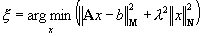
Taking into account the measurement noise n, supposed to be normally distributed, an estimate of the dipole source configuration that generated a measured potential b can be obtained by solving the linear system:

                                                                                                                       (1)

where A is a matrix with number of rows equal to the number of sensors and number of columns equal to the number of modeled sources, called lead field matrix. The electrical lead field matrix A and the data vector b must be referenced consistently. Among the several equivalent solutions for the underdetermined system (1), the solution was chosen that satisfies the following variational problem for the sources x (Dale and Sereno, 1993; Grave de Peralta and Gonzalez Andino, 1998; Liu, 2000):

                                                                                       (2)

where M, N are the matrices associated to the metrics of the data and of the source space, respectively. The solution of the variational problem depends on adequacy of the data and source space metrics. Under the hypothesis of M and N positive definite, the solution of eq. 2 is given by computing the pseudoinverse matrix G according to the following expressions:

,                                                                             (3)

An optimal regularization of this linear system was obtained by the L-curve approach (Hansen, 1992). This curve, which plots the residual norm versus the solution norm at different l values, was used to choose the optimal amount of regularization in the solution of the linear inverse problem. Computation of the L-curves and optimal l correction values was performed with the original Hansen’s routines (Hansen, 1994). The metric M, characterizing the idea of closeness in the data space, can be particularized by taking into account the sensors noise level by using the Mahalanobis distance (Grave de Peralta and Gonzalez Andino, 1998). The source metric N can be particularized by taking into account the information from the hemodynamic responses of the single voxels, as showed in the following section.

Functional hemodynamical coupling and linear inverse estimation of source activity

Here, we present two characterizations of the source metric N that can provide the basis for the inclusion of the information about the statistical hemodynamic activation of i-th cortical voxels into the linear inverse estimation of the cortical source activity. The first characterization of the source metric N takes into account all the cortical voxels on the basis of their electrical “closeness” to the EEG sensors (column norm normalization; Pascual-Marqui et al., 1994; Gorozdnistky et al., 1995; Grave de Peralta and Gonzalez Andino, 1998). In this case, the inverse of the resulting source metric is

                                                                                                             (4)

in which  is the i-th element of the inverse of the diagonal matrix N and  is the L2 norm of the i-th column of the lead field matrix A.

Introducing fMRI priors into the linear inverse estimation produces a bias in the solution: statistically significantly activated fMRI voxels, which are returned by the so called percentage change approach (Kim et al., 1993), are weighted to account for the EEG measured potentials. The inverse of the resulting metric is

                                                                                                (5)

in which  and  has the same meaning described above. The  is a function of the statistically significant percentage increase of the fMRI signal assigned to the i-th dipole of the modeled source space. This function was expressed as

,     ,                                                       (6)

where  is the percentage increase of the fMRI signal during the task state for the i-th voxel and the factor K tunes fMRI constraints in the source space. Fixing K = 1 let us disregard fMRI priors, thus returning to a purely electrical solution; a value for K >> 1 allows only the sources associated with fMRI active voxels to participate in the solution. It was shown that a value for K in the order of 10 (90% of constraints for the fMRI information) is useful to avoid mislocalization due to over constrained solutions (Liu et al., 1998; Dale et al., 2000; Liu, 2000). In the following the estimation of the cortical activity obtained with this metric will be denoted as diag-fMRI.

The previous definition of the source metric N results in a matrix in which the off-diagonal elements are zero (diag-fMRI). However, we can take advantage of the off-diagonal elements of the matrix N to insert the information about the functional coupling of the cortical sources. In particular we set the generic ij entry of the inverse of matrix N as in the following

                                                                   (7)

where  and  have the same meaning described above and  is the degree of functional coupling between the source i and the source j during the particular task analyzed. Such coupling was revealed by the correlation of their hemodynamic responses obtained by the event-related fMRI data. In the following the estimation of the cortical activity obtained with this metric will be denoted as corr-fMRI. It is of interest that in the case of uncorrelated sources (, ; ), the corr-fMRI formulation leads back to the diag-fMRI one. Fig.1 summarizes the different approaches pursued here in order to insert the hemodynamical constraints in the solution of the linear inverse problem for the estimation of the cortical sources of the recorded EEG in a unique mathematical formulation.

Figure 1.  Upper part: Estimate of the hemodynamic coupling between two generic cortical sources (i-th and j-th) as obtained by the computation of the cross-correlation between the waveforms of the fMRI responses. These waveforms (Si, Sj) were obtained  during a simple voluntary movement (right middle finger extension). Lower part: mathematical formulation of the inverse of the source metric N to be used in the solution of the linear inverse problem. Corr(Si,Sj) is the zero-lag correlation between the two hemodynamic waveforms Si and Sj, and is the Kroneker symbol.

EEG recording

EEG activity was recorded (0.1-100 Hz bandpass) with 128 electrodes (linked earlobe electrical reference). Electrode positions and reference landmarks were digitized for subsequent integration between the EEG, MEG, and MR data. Electrooculogram (EOG; 0.1-100 Hz bandpass) and electromyogram (EMG; 1-100 Hz bandpass) from m. extensor digitorum of both sides were also recorded. EOG served to control blinking/eye movements and EMG to control operating muscle response and involuntary mirror movements. All data were acquired (400 Hz sampling rate) from 3 sec before to 1 sec after the onset (zerotime) of the EMG response from the operating muscle. About 200 single trials were collected and averaged for each subject.

3. Results and Discussion

Fig. 2 illustrates the topographic map of readiness potential distribution recorded at the scalp about 200 ms before a right middle finger extension (subject #1). Note the extension of the maximum of the negative scalp potential distribution, roughly overlying frontal and centroparietal areas contralateral to the movement. Fig.2 illustrates also the percent values of the fMRI response during the movement in a separate experimental session. The maximum values of the fMRI responses are located in the voxels roughly corresponding to the primary somatosensory and motor areas (hand representation) contralateral to the movement.

 

Figure 2.  Left: scalp potential distribution recorded about 200 msec before the movement onset (128 recording channels) in a separate session. This distribution is representative of the so called readiness potential. Percent color scale in which maximum negativity (-100%) is coded in red and maximum positivity (+100%) is coded in black.. Right: fMRI response related to the movement in subject 1. Only the brain voxels whose hemodynamic response is increased statistically are shown. The fMRI response is integrated to a MRI-based reconstruction of the cortical surface. The red to yellow color bar codes  the percentage of the increase of the fMRI response

Fig. 3 illustrates the cortical distribution of the current density estimated with linear inverse approach from the potential distribution of Fig.2. Such an approach used no-fMRI constraint as well as two types of fMRI constraints, i.e. one based on block-design (diag-fMRI) and the other on event-related design (corr-fMRI). The cortical distributions are represented on the realistic subject’s head volume conductor model.  Linear inverse solutions obtained with the fMRI priors (diag and corr-fMRI) present more localized spots of activations with respect to those obtained with the no fMRI priors. Remarkably, the spots of activation were localized in the hand region of the primary somatosensory (post-central) and motor (pre-central) areas contralateral to the movement. In addition, spots of minor activation were observed in the frontocentral medial areas (including supplementary motor area) and in the primary somatosensory and motor areas of the ipsilateral hemisphere.  Similar results were obtained in the other main components of the movement-related potentials (i.e. motor potentials and movement-evoked potential) and in the other subject.

Figure 3. Cortical distributions of the current density estimated with a linear inverse approach from the readiness potential of Fig.2. Linear inverse estimates are obtained with no fMRI constraints (no-fMRI) and two kinds of fMRI constraints, one based on the strengths of the cortical fMRI responses (diag-fMRI) and the other on the correlation between fMRI responsive cortical areas (corr-fMRI). Percent color scale: maximum negativity (-100%) is coded in red and maximum positivity (+100%) is coded in black.

The results of the present study are in line with those regarding the coupling between cortical electrical activity and hemodynamic measure as indicated by a direct comparison of maps obtained using voltage-sensitive dyes, which reflect depolarization of neuronal membranes in superficial cortical layers, and maps derived from intrinsic optical signals, which reflect changes in light absorption due to changes in blood volume and oxygen consumption (Shoham et al., 1999). Furthermore, previous studies on animals have also shown a strong correlation between local field potentials, spiking activity, and voltage-sensitive dye signals (Arieli et al., 1996). Finally, studies in humans comparing the localization of functional activity by invasive electrical recordings and fMRI have provided evidence of a correlation between the local electrophysiological and hemodynamic responses (Puce et al, 1997). This may suggest that the local fMRI responses can be reliably used to bias the estimation of the electrical activity in the regions showing a prominent hemodynamic response.

It may be argued that combined EEG-fMRI responses could be less reliable for the modeling of cortical activation in the case of a spatial mismatch between electrical and hemodynamical responses. However, previous studies have suggested that by using the fMRI data as a partial constraint in the liner inverse procedure, it is possible to obtain accurate source estimates of electrical activity even in the presence of some spatial mismatch between the generators of EEG data and the fMRI signals (Liu et al., 1998; Liu, 2000). Furthermore, it is questionable if  the level of the bias for the hemodynamical constraints in the linear inverse estimation can be the same with the diag-fMRI and corr-fMRI approaches, (so did we in this present study). We think that this issue deserves a specific simulation study, using the literature indexes capable of assessing the quality of the linear inverse solutions (Pascual Marqui et al., 1994; Grave de Peralta and Gonzalez Andino, 1998, Babiloni et al., 2001).

In conclusion, the present paper dealt with the issue of combining fMRI and EEG data for the study of event-related cortical responses. This approach can be further enriched incorporating magnetoencephalographic data in the linear inverse estimation, to constitute an unsurpassable non invasive technology for the analysis of human higher brain functions at a high temporal and a good spatial resolution.

References